Author: Ciamac Moallemi, Dan Robinson, Paradigm
Compiled by: Yangz, Techub News
Introduction
In this article, we introduce a new type of automated market maker (AMM) tailored for prediction markets: the pm-AMM.
AMMs and their predecessors (such as market scoring rules) were originally invented as a way to provide liquidity for prediction markets. They now dominate the trading volume of most DEXes. However, ironically, while prediction market trading volumes have skyrocketed, most of them use order books rather than AMMs.
One possible reason is that existing AMMs are not well-suited for outcome tokens (i.e., tokens that are worth $1 if an event occurs and $0 if it does not). The volatility of outcome tokens depends on the current probability of the event and the time to expiration of the prediction market, meaning that the liquidity provided by the liquidity pool is inconsistent. Once the prediction market expires, the liquidity providers (LPs) essentially lose all their value.
To address this, we propose a new type of AMM optimized around these considerations, aiming to solve a long-standing problem in AMM research: what does it mean to optimize an AMM for a particular class of assets? In other words, given a model for some asset (e.g., options, bonds, stablecoins, or outcome tokens), how would that affect the AMM we would apply? We offer a potential answer to this question based on the concept of loss versus rebalancing (LVR).
Findings
We establish a model for the price dynamics of some outcome tokens, which we call the Gaussian score dynamics. This model may be applicable to prediction markets that aim to predict whether certain basic random walks (e.g., the score difference in a basketball game, the vote difference in an election, or the price of some asset) will be above a certain value at a future expiration time.
Using this model, we derive a new invariant-based AMM for these tokens, the static pm-AMM invariant:
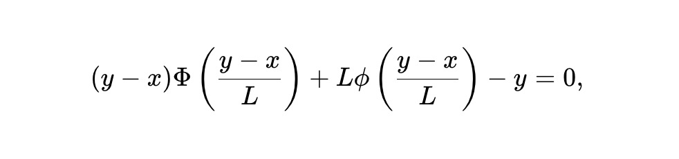
where x is the reserve of the outcome token in the AMM, y is the reserve of the opposing/complementary outcome token, L is the overall liquidity or scale factor, and ϕ and Φ are the probability density function and cumulative distribution function of the normal distribution, respectively.
This invariant is based on a powerful concept called loss versus rebalancing (LVR), which we can think of as the rate at which the AMM loses due to arbitrage, and which depends on the shape of the AMM and the price movements of the related assets traded on the AMM.
We define a uniform AMM for an asset as one where, if used for that asset, the LVR is proportional to the portfolio value at any given time, regardless of the current price. Milionis et al. show that for assets whose prices follow geometric Brownian motion (GBM, a popular model for the price dynamics of ordinary assets like stocks and cryptocurrencies), the constant-product market maker (like Uniswap and Balancer) is the unique uniform AMM, and the static pm-AMM is the uniform AMM for assets whose behavior follows the Gaussian score dynamics we propose for outcome tokens.
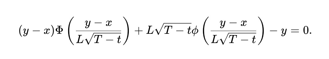
While the static pm-AMM has a uniform LVR (as a fraction of the portfolio value) at all prices, the LVR still increases as the prediction market approaches expiration. This is because prediction markets can become highly volatile near expiration. To adjust the pm-AMM to reduce its liquidity, thereby keeping the expected LVR constant across all times until expiration, we derive the dynamic pm-AMM invariant, which depends on the time to expiration T-t:
The dynamic pm-AMM mechanism provides decreasing liquidity over time to prevent the LVR from increasing as expiration approaches. In a real-world liquidity pool, this may not be desirable, especially since non-arbitrage trading activity (and the resulting fees) may also increase over time. However, the pm-AMM provides a framework for liquidity providers to adjust the liquidity based on their expected fees and how they wish to allocate the arbitrage risk.
These AMMs may help guide the passive liquidity on-chain prediction markets. The concept of uniform AMMs and the associated techniques may also be more broadly applicable to DEX designers who wish to customize AMMs for other asset types whose price dynamics do not follow geometric Brownian motion, such as stablecoins, bonds, options, or other derivatives.
Figure 1 shows the invariant curves of the static and dynamic pm-AMMs, and compares them to other well-known invariant curves, namely the constant-product market maker (CPMM) and the logarithmic market scoring rule (LMSR). Note that the reserve curve of the dynamic pm-AMM provides lower liquidity over time.
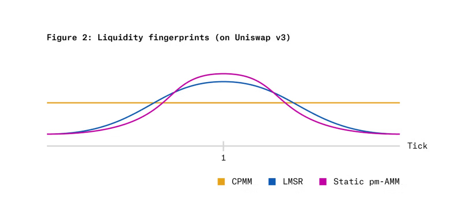
Figure 2 shows the "liquidity fingerprint" that would result if the static pm-AMM invariant were implemented on a Uniswap v3 concentrated liquidity AMM, compared to CPMM and LMSR. The x-axis corresponds to a log scale of the relative price (the price of the x token divided by the price of the y token), and the y-axis corresponds to the liquidity concentrated at each price level by each AMM. We can see that, compared to these two alternatives, the pm-AMM concentrates more liquidity around the relative price of 1 (50% probability, i.e., the token prices are equal to 0.50) and less liquidity at extreme relative prices (very low or very high).
Background
Prediction Markets
Prediction markets are a growing application in the cryptocurrency space. In October 2024 alone, Polymarket's trading volume exceeded $2 billion. However, most cryptocurrency prediction markets provide liquidity through order books rather than AMMs, despite the latter dominating the trading volume of most DEXes.
One possible reason is that the price behavior of outcome tokens is different from ordinary assets, so AMMs designed for them cannot operate stably. For example, imagine a prediction market for a coin-flipping game, where 1001 coin flips are performed, and each outcome (heads or tails) corresponds to x and y tokens, respectively. Ultimately, if heads come up more, the x token is worth $1, and if tails come up more, the x token is worth $0; the y token is the opposite.
The volatility of these outcome tokens depends heavily on the remaining number of flips and the current state of the flips. The closer the current state is to even, and the fewer remaining flips, the higher the volatility of these tokens. This means that the losses (which depend on volatility, as discussed below) of a constant-product market maker vary greatly over time.
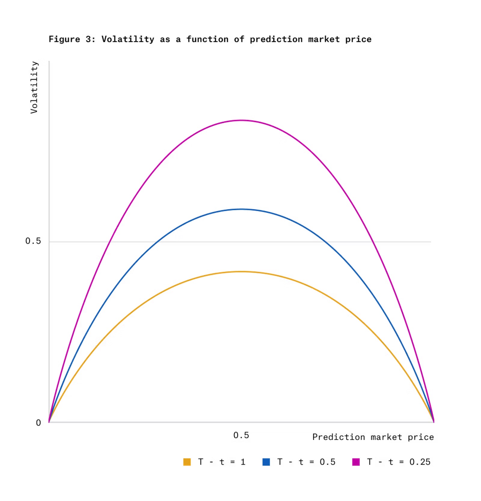
Figure 3 shows the relationship between the volatility of outcome token prices and the token prices and remaining time under the Gaussian score dynamics.
Many popular prediction markets are actually similar to this coin-flipping example, betting on whether a random walk will end up above or below 0 at a future expiration time. For example:
A prediction market on the outcome of a basketball game would expire when the game clock reaches 0. The random walk is the score difference between the two teams.
A prediction market on the outcome of a presidential election would expire on election day. The random walk is the difference in the number of voters intending to vote for each candidate.
A prediction market on whether the price of an asset like Bitcoin will be above a strike price on a future date, the random walk could be the log of the current Bitcoin price minus the strike price.
The inspiration for the Gaussian score dynamics model we define for outcome token price movements comes from these types of examples. The model assumes that the prediction market price matches the probability that the underlying Brownian motion ends up above 0. It is similar to the Black-Scholes model for binary options (which pay a fixed dollar amount if the asset price is above a strike, and 0 otherwise), but our model does not require the underlying process to correspond to a tradable asset price.
We have indeed made a simplifying assumption that the price of the outcome token matches the probability of it being $1. This assumption ignores important features of the market, including risk and time preferences, and studying how these features affect this model will be a subject for future research.
Additionally, we should also recognize that not all prediction markets are suitable for the Gaussian score dynamics model, as the model assumes a predictable speed of new information arrival. For example, basketball games may be more suitable for this model than soccer games, as the scoring frequency is much higher in basketball, and hence the evolution of the score difference over time will also be more consistent. Furthermore, some types of prediction markets are completely different from this model, such as predicting whether a one-time event (such as an earthquake) will occur before a specific date. However, the model may be a useful starting point for deriving other dynamic models, and can serve as a demonstration of a method for deriving a unified AMM for any model.
Loss vs Rebalancing and Uniformity
After establishing this model, we have derived a mechanism that may be more suitable for these tokens than existing AMMs (such as constant product market makers or LMSR). The guiding metric we use is the expected loss rate of liquidity providers, which can be characterized as "loss-vs-rebalancing" or LVR.
LVR captures the main adverse selection cost of AMMs: in the absence of trades, the AMM's prices are static, while new information causes the prices to become stale. LVR reflects the cost borne by AMM liquidity providers, as these stale prices are exploited by more informed arbitrageurs who trade at prices unfavorable to the AMM. Thus, LVR can be viewed as the fee the AMM pays to arbitrageurs to correct its prices.
Furthermore, in the absence of trading fees, LVR is also the loss incurred by liquidity providers when they delta-hedge their LP position by holding a short position in the tokens separate from the pool reserves. Thus, LVR is built on the key insights of the Black-Scholes option pricing model. Just as options eliminate market risk through delta-hedging against the underlying asset, LVR values the LP position in the AMM after eliminating market risk. That is, LVR isolates the special nature of being a liquidity provider in an AMM, rather than simply bearing the market risk of holding the same tokens as the AMM reserves.
We consider simple invariant-based AMMs without fees or MEV capture mechanisms. In this case, the AMM must lose to arbitrage, and no AMM invariant can eliminate LVR (except for invariants that fundamentally do not generate any trades). Furthermore, even "minimizing" LVR has no practical meaning, as reducing LVR only means reducing the liquidity provided.
However, while we cannot eliminate LVR, we can make LVR more uniform, so that the percentage loss of the asset pool value does not depend on the current price of the asset. We call this property uniformity.
Imagine a sponsor willing to provide liquidity on a zero-fee prediction market to understand the market's prediction of the outcome. The sponsor will lose money, but it is also more willing to spread the loss evenly rather than concentrating the loss at specific times or prices. In this case, the current portfolio value of the asset pool can be viewed as the sponsor's "budget". On a uniform AMM, if the sponsor injects $1 of liquidity at some time, their expected loss at the next time point is independent of the current state of the fund.
Furthermore, uniformity has potential significance for profit-seeking liquidity providers as well. Even if the AMM can capture some of the gains from loss-vs-rebalancing, or even turn a profit (through non-zero swap fees, or auction mechanisms like MEV taxes), it still needs some strategy to determine how to allocate liquidity across different prices and times. We can view the expected loss of the zero-fee pool as a way to measure this strategy, taking into account the price process of the asset.
We define a uniform AMM for a given asset as an AMM where the expected LVR is a constant fraction of the current value of the asset pool, regardless of the current price of the asset. Note that whether an AMM has a uniform LVR depends on the price process of the asset itself. As shown in Appendix B.2 of Milionis et al., if the asset's price follows a geometric Brownian motion, then the essentially unique uniform AMM for that asset is the weighted geometric mean market maker, with the invariant:
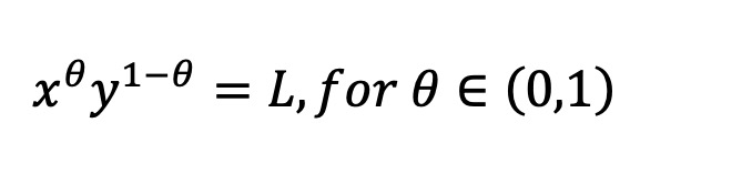
This is the formula used in Balancer, and the constant product market maker used in Uniswap v2 is a special case of it. However, for tokens following Gaussian score dynamics, the constant geometric mean AMM does not have a uniform LVR. The logarithmic market scoring rule (LMSR) is also the case.
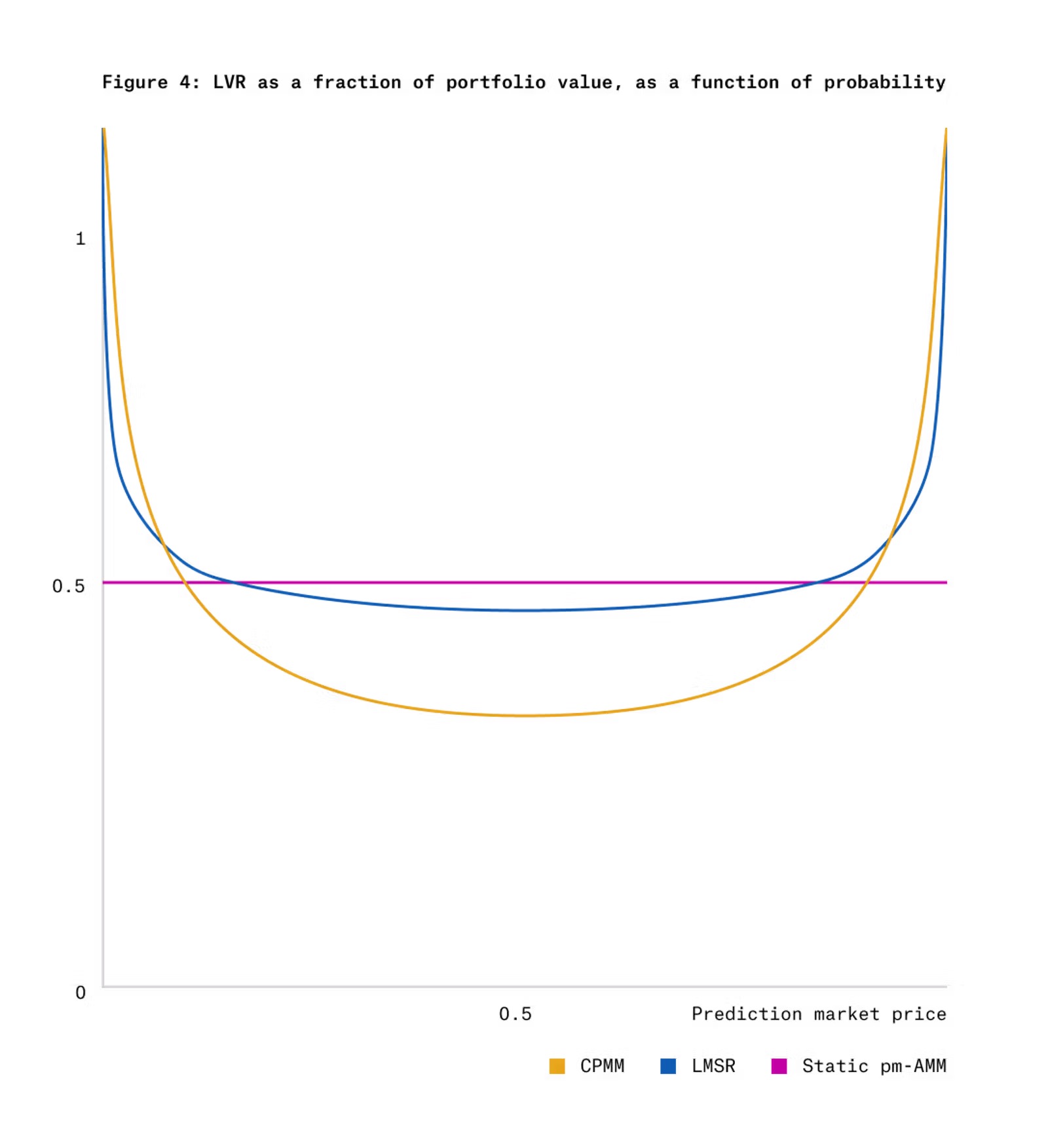
Figure 4 shows the LVR for CPMM and LMSR compared to the uniform LVR of the static pm-AMM for Gaussian score dynamic outcome tokens at time T-t=1.
Considering these factors, we have developed two AMMs designed for prediction markets under Gaussian score dynamics: one that has a uniform LVR at any given time, but the LVR increases as the prediction market approaches expiration; and another that has a uniform LVR and constant expected LVR over the remaining time range.
As shown in Figure 4, CPMM and LMSR exhibit larger LVRs when the outcome token price is in the extreme near-zero or near-one regions. This is because, while price volatility is lower around these points (see Figure 3), the rate of decay of the asset pool value is faster at extreme prices. Therefore, the uniform AMM should provide less liquidity at extreme prices, which is precisely what the pm-AMM design does (see Figure 2).
Prior Work
AMMs originate from prediction markets and market scoring rules (such as LMSR). These rules led to the discovery of constant function market makers (CFMMs), such as Uniswap v2, which typically have an invariant relationship between the reserves of each asset. AMMs based on this design have become the mainstream market mechanism for DEXes in recent years.
Recently, perspectives from financial economics have been applied to understand the costs of automated market makers, in the form of loss-vs-rebalancing (LVR), primarily focusing on geometric Brownian motion. On the other hand, the price dynamics of prediction markets are very different, as their payoffs are bounded and have finite horizons. Taleb proposed dynamics based on the potential observable voting process, while we have developed another based on a potential observable Gaussian score process.
There have been some applied research on designing automated market makers for non-GBM assets. One example is StableSwap, an AMM designed for stablecoin pairs, based on the intuitive premise that the AMM between correlated assets and mean-reverting assets should tightly concentrate liquidity around a single price, but its derivation does not involve modeling the asset price process. Another example is YieldSpace, an AMM designed for zero-coupon bonds. While the YieldSpace derivation does involve a simple zero-coupon bond pricing model, it does not include a full price process model (no modeling of the evolution of interest rates).
Additionally, there has been some academic work on designing real-time market models around beliefs about asset price behavior. One example is the design by Goyal et al. Their framework is designed around maximizing expected active liquidity, rather than making expected losses uniform, and thus sometimes reaches conclusions opposite to ours. For example, they derive that if liquidity providers expect the relative price of an asset to stay around 1, then LMSR (which concentrates liquidity around price 1) is very suitable, whereas our framework suggests that if the expected price is to become polarized (like outcome tokens), there is a rationale to concentrate liquidity around 1.
Different AMM Models
Automated Market Makers
We can consider a prediction market for a single event, and an AMM that trades two competing assets. One risky asset, denoted by x, pays $1 if the event occurs, and 0 otherwise; the other risky asset, denoted by y, has the opposite payoff. The AMM maintains an invariant f(x,y)=L, where f(⋅,⋅) is an invariant function of the reserves (x,y), and L is a constant. Given the price P of the x asset in dollars, the value function of the asset pool is:
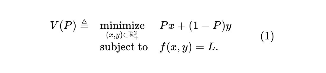
This is the value of the asset pool when the price of x is P. Since holding one unit of x and y assets is equivalent to holding cash, we must set the price of y to 1-P. Assume there is a group of arbitrageurs who can observe the price of the x asset Pt (as well as the price of the y asset 1-Pt) at each time t. Assuming no transaction costs or other frictions, these arbitrageurs will continuously monitor the AMM and attempt to extract value from any mispricing in the AMM. In pursuit of their own profit maximization, they will trade against the AMM to minimize the value of the AMM's reserves. If we denote the reserve value at time t (when the price is Pt) as Vt, then Vt = V(Pt).
Example 1: In the case of a Constant Product Market Maker (CPMM), the invariant is f(x,y)≜xy, and the asset pool value function is:

Example 2: The Logarithmic Market Scoring Rule (LMSR) created by Robin Hanson can be viewed as an AMM that satisfies the following invariant.
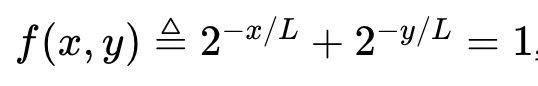
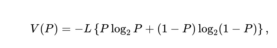
Its asset pool value function is (proportional to the binary entropy implied by the price):
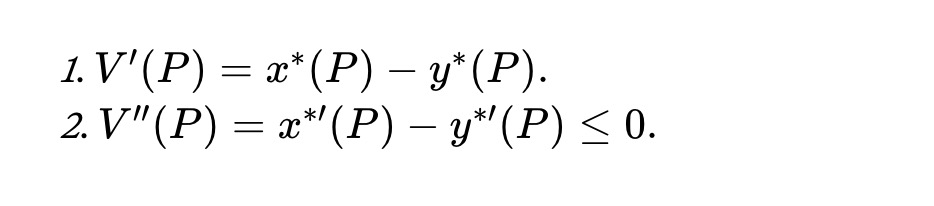
Let x∗(P) and y∗(P) denote the optimal solutions to the optimization problem (1), and assume they exist, are unique, and are sufficiently smooth functions of the price P. Then the following formula is similar to Theorem 1 of Milionis et al., but applicable to the current setting:
Theorem 1. For all prices P≥0, the asset pool value function satisfies:
Gaussian Score Dynamics
How does the price of the risky asset evolve over time according to the Gaussian score dynamics we described? Specifically, we assume that there exists a stochastic process {Zt} on the time interval t∈[0,T], where the event is determined by the sign of ZT at the end of the time span t=T: if ZT≥0, the x asset pays out, and if ZT<0, the y asset pays out. We can think of Zt as the score difference between the two competing teams. Note that while our model assumes the existence of this score process, the AMM does not need to directly observe these processes. As discussed below, the AMM can infer the current value of the score based on the marginal prices (after arbitrage) and the time to maturity.
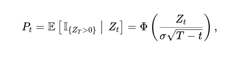
We assume that Zt follows a random walk. Specifically, we assume that Zt is a Brownian motion with volatility σ>0, i.e., dZt=σdBt, where Bt is a standard Brownian motion. Then, it is not difficult to see that the price of the x asset at time t, Pt, is:

where Φ(⋅) is the standard normal cumulative distribution function (CDF). Applying Itô's lemma, Pt must satisfy:
where ϕ(⋅) is the standard normal probability density function, and Φ-1(⋅) is the inverse CDF. Note that while the score dynamics and the transformation from scores to prices or vice versa depend on σ, the isolated price process Pt dynamics do not depend on σ. The volatility of these dynamics as a function of price and remaining time is shown in Figure 3.
Unified AMM
Based on the discussion above, if we denote the value of the asset pool reserves at time t as Vt, then Vt=V(Pt). Applying Itô's lemma, we can derive that the asset pool value evolves according to the following formula:
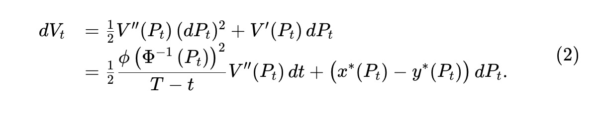
Since the price Pt is a martingale, the second term in (2) is also a martingale, which may be increasing or decreasing. However, according to V(⋅) (see Theorem 1), the first term corresponds to a negative drift, and thus is a decreasing process. This is the loss and rebalancing process proposed by Milionis et al., which captures the value lost by arbitrageurs who hedge against the asset pool at unfavorable prices. We define the instantaneous rate of this loss as:
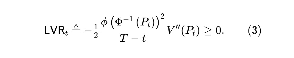
Milionis et al. found that for assets following geometric Brownian motion, only the geometric mean market maker is a unified AMM. In prediction markets with Gaussian score dynamics, to examine (3), a unified LVR pool must solve the following ordinary differential equation (ODE):
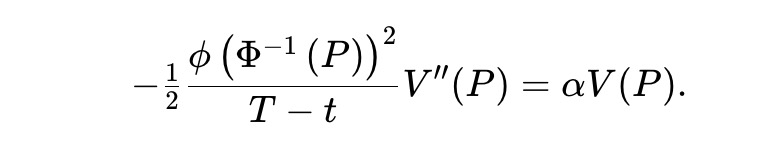
This is impossible, as the left-hand side depends on t, while the right-hand side does not depend on t. The core issue here is that the dynamics of geometric Brownian motion are time-invariant, while the Gaussian score dynamics are highly time-dependent.
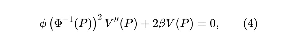
To circumvent this problem, we allow α to be time-dependent, i.e., we can set α=β/(T-t), where β>0, and consider the following setting:

This is equivalent to an ODE for P≥0. Additionally, V(⋅) has some further requirements, such as V′′(P)≤0 (see Theorem 1).
Static pm-AMM
The above ODE can be simplified by changing the variable to u=Φ-1(P). When β=1/2, there is a solution that satisfies the ODE and the additional concavity requirement, which is:

The reserves of the x and y tokens are:
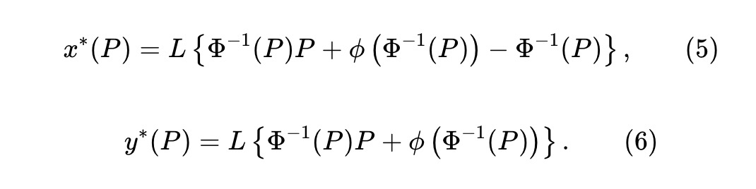
Here, L≥0 is a liquidity parameter that determines the scaling of the pool size. Observing y∗(P)-x∗(P)=LΦ-1(P) and substituting it into (5), the pool reserves (x,y) must satisfy the invariant:
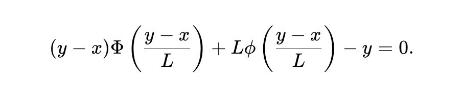
This is the definition of the static pm-AMM. By design, this AMM satisfies the following relationships:

Define Vˉt=E[Vt] as the expected pool value, and from (2) we can derive:

Solving this ordinary differential equation, we can obtain the following solution. In other words, in the expected case, the asset pool value of the static pm-AMM decays with the square root of the remaining time range.

Dynamic pm-AMM
A drawback of the static pm-AMM is that while its LVR per dollar value is unified across all possible prices, it changes over time. Specifically, the loss per $1 value is inversely proportional to the time to maturity, so it will increase over time until it loses all value at maturity.
Dynamic Liquidity. We envision a time-varying dynamic version of the static pm-AMM design, where AMM LPs extract liquidity over time to reduce losses. Specifically, assume the pool value is:

where Lt is a deterministic, smooth function that determines the degree to which liquidity is removed (or potentially added) over time. Applying Itô's lemma to the asset pool value process Vt≜V(Pt,t), we have
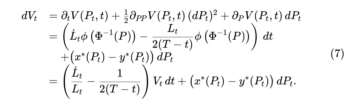
Let Ct denote the cumulative dollar value of liquidity extracted. Since the pool value is linearly related to the liquidity Lt, the dollar value of the change in Lt is proportional to Vt/LT. We can obtain:

The total wealth Wt of the AMM LPs consists of the value of the pool reserves and the cumulative value of the extracted liquidity, so Wt=Vt+Ct, and satisfies:
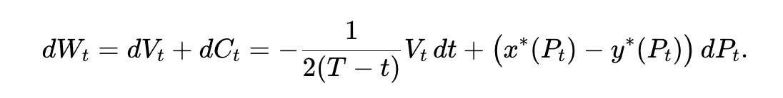
This means that the expected wealth Wˉt≜E[Wt] of the LPs satisfies the following, where Vˉt≜E[VT].

Now, consider the specific choice of the liquidity curve:

We call it dynamic pm-AMM. According to (7), the expected asset pool value Vˉt=E[Vt] satisfies:
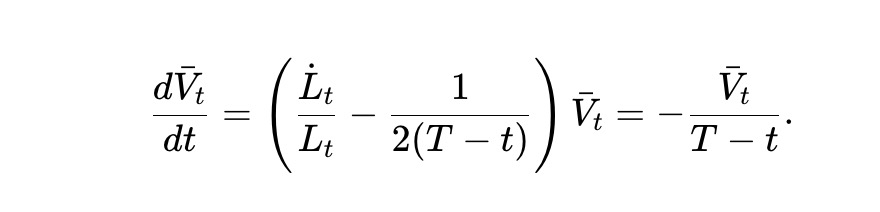
Solving this ordinary differential equation, we can obtain the following answer.

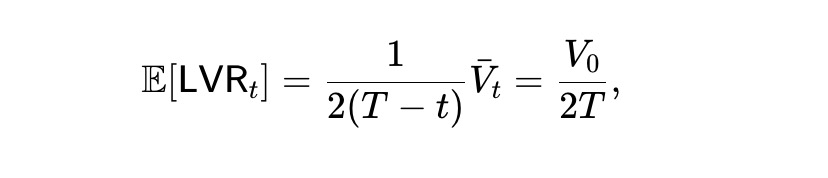
In other words, in the dynamic pm-AMM, the expected fund pool value decreases linearly after withdrawal. Furthermore, due to inheriting the value function of the static pm-AMM, the LVR loss rate per unit time is:

The expected loss rate is the following value, which remains constant during the period t. That is, over time, the dynamic pm-AMM will (expectedly) lose the arbitrageur's funds at a constant speed.
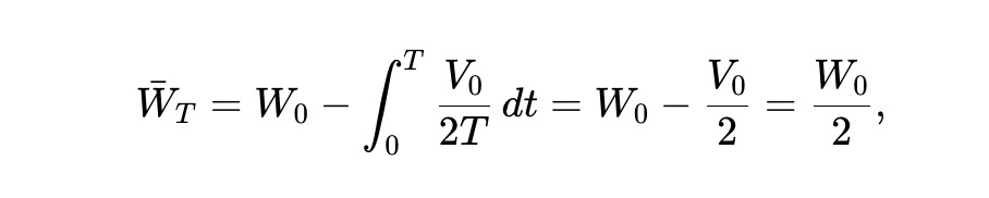
Finally, according to (8), the expected wealth process is shown in the figure below. Therefore, half of the initial wealth will be lost in the end.
Conclusion
pm-AMM may be applicable to prediction markets driven by dynamic models such as Gaussian diffusion dynamics. In addition, our research also suggests that unified AMM may be applicable to other types of assets, such as bonds, options, and other derivatives.