Author: Dmytro Zakharov
Acknowledgments
This work is based on research I conducted during my time at Blockstream's research department . Thank you all for your support and for giving me the opportunity to research this topic.
Special thanks to Jonas Nikc for his meticulous review of this article and his very helpful suggestions; and to Mykyta Redko for pointing out several important errors in the explanations.
introduction
The publication of Google Quantum AI's latest paper has reignited discussions about when the first "cryptographically secure quantum computer (CRQC)" will be available (frankly, in some places, it has even turned into a panic). Opinions differ greatly, but one point seems to be agreed upon by everyone: we need to migrate to quantum-safe algorithms as soon as possible.
Of course, this is necessary for many protocols already in service; in particular, in Bitcoin (and the broader blockchain space), the natural first step is to construct a post-quantum (PQ) secure electronic signature scheme. However, even this first step involves much controversy: there are many alternative PQ schemes, but they are all (a) significantly worse than the “dispersed logarithm (DL)” construction on certain metrics (at least 16 times); and (b) the underlying security assumptions are generally less studied (compared to pre-quantum equivalents).
Currently, PQ signatures mainly fall into two categories: hash function-based and lattice-based . Blockstream has produced a wealth of analysis and research on hash function-based cryptography: for example, " Considering Hash Function-Based Signature Schemes for Bitcoin " by Jonas Nick and Mikhail Kudinov, and the SHRIMPS scheme proposed by Jonas Nick. Now, it's time for lattice-based construction!
Important Reminder
We note that there are also code-based constructs, but their public keys and signatures are too large: for example, the smallest public key size for LESS, a major (former) NIST candidate, is 13.9KB. That said, at present, it doesn't seem to be a viable option for Bitcoin.
The topic of this article
As mentioned earlier, we are prepared to analyze the fundamental ideas behind lattice-based signature schemes. In particular, after reading this article, readers will gain a solid understanding of a key technique called "Fiat- Shamir with aborts " (also known as " refusal sampling "), which is used in Dilithium and, for example, many lattice-based proving systems (see " Lattice-Based Product Proofs "). Surprisingly, this technique is very similar to the construction of traditional Schnorr signatures based on the discrete logarithm assumption. In this article, we will provide a set of basic tools to help readers understand lattice-based schemes, hoping to make it easier for them to enter this field of cryptography.
More specifically, in this article, we will start with the famous paper " Trapdoor-Free Lattice Signatures " to understand the construction proposed by the author Lyubashevsky; this paper is probably the most influential in the entire field of lattice cryptography.
Basic introduction to grids
grid
Let me first introduce our research object. We define an $m$-dimensional "lattice" $\Lambda \subseteq \mathbb{R}^d$ as all integer linear combinations of a set of independent linear vectors $\mathbf{b}_1,\dots,\mathbf{b}_m$ over $\mathbb{R}^d$ (d-dimensional real space), that is:
$$
\begin{equation*}
\Lambda \triangleq \left{ \sum_{i=1}^m \lambda_i\mathbf{b}_i: \lambda_1,\dots,\lambda_m \in \mathbb{Z} \right}.
\end{equation*}
$$
To understand this more intuitively, here is a concrete example: The image below is a two-dimensional (m=d=2) lattice.
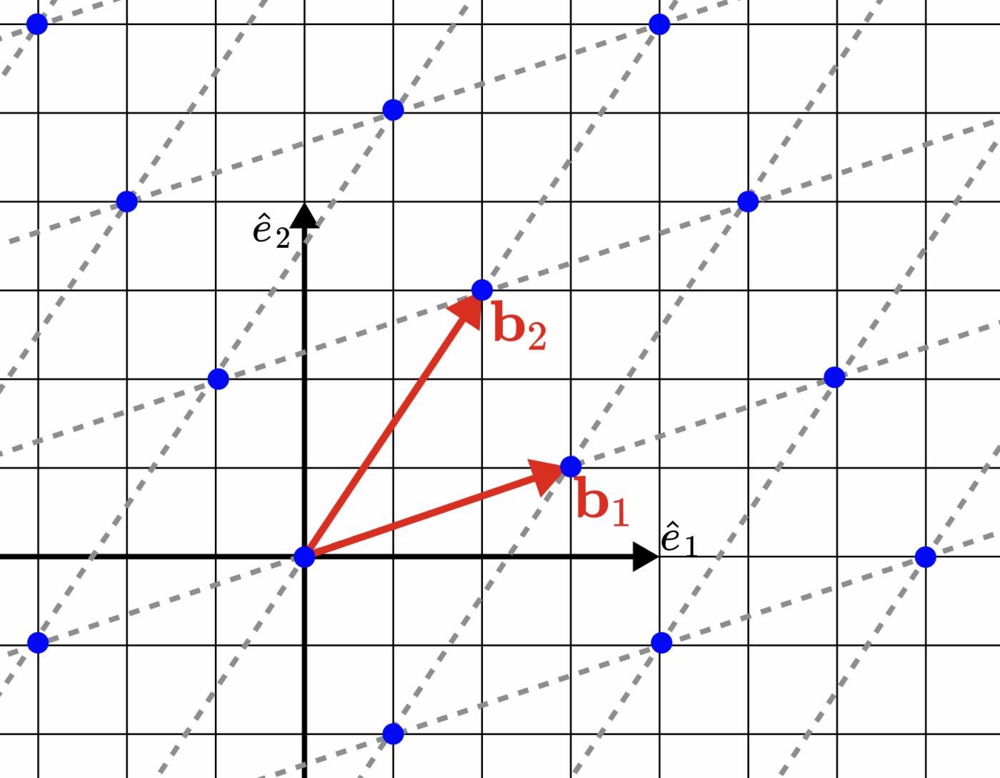
Figure 1. An example of a two-dimensional lattice spanned by vectors $b_1 = (3, 1)$ and $b_2 = (2, 3)$. The resulting lattice $\Lambda$ is a set of blue points.
When I first read this definition, I couldn't help but wonder, "What useful information could such a straightforward definition possibly provide?" However, long before cryptographers noticed that lattices were the root fields of many computationally difficult problems, they had already been proven mathematically useful, dating back at least to the 18th century. In fact, lattices naturally appear in many fields, such as number theory and the sphere packing problem (both of which are more or less related to lattice-based and code-based cryptography).
Note:
Sometimes I hear the statement, "Latticees are far too immature compared to hash-based cryptography." However, this is a misconception, as lattices were used and studied long before hash functions were invented (dating back to around 1950). :) Nevertheless, lattices do possess a richer algebraic structure than hash functions. While this can lead to more advanced cryptographic protocols (e.g., multi-signatures or SNARKs), we must still be cautious about their security.
Lattice problem in cryptography
Lattice-based cryptography revolves around a set of assumptions that can be reduced to solving problems on lattices $\lambda$. These problems, in turn, are currently considered unsolvable even by quantum computers. Many such assumptions exist, including: the Shortest Vector Problem ( SVP ), the Closest Vector Problem ( CVP ), Finite Distance Decoding ( BDD ), the Lattice Isomorphism Problem ( LIP ), the Deterministic Shortest Vector Problem ( GapSVP ), and so on.
In this article, we will only introduce one of the assumptions.
The (approximate) shortest vector problem ($\gamma$-SVP) aims to find a "very short" vector on the lattice $\Lambda$. We can (relatively easily) prove that $\Lambda$ contains this shortest vector (i.e., there exists $\mathbf{u} \in \Lambda$ such that $|\mathbf{u}|=\min_{\mathbf{v} \in \Lambda}|\mathbf{v}|$, whose length we denote as $\lambda_1(\Lambda)$. However, finding such a vector is considered a difficult problem even for quantum computers. We call this problem " SVP ".
However, developing a practical protocol based on this "naked" SVP is nearly impossible. Therefore, we relax the requirements: assuming we accept vectors whose norm is less than $\gamma\lambda_1(\Lambda)$, it only requires that the factor $\gamma>1$. It can be proven that such a modified problem remains difficult enough even for large factors, such as $\gamma=\mathsf{poly}(\sqrt{d})$. This modified problem is called "$\gamma$ -SVP ". (Translator's note: A norm is a function that maps vectors in a vector space to real numbers. In other words, each norm corresponds to a way of defining the length of a vector; the norm value can be understood as length.)
This problem can be illustrated with the following diagram.
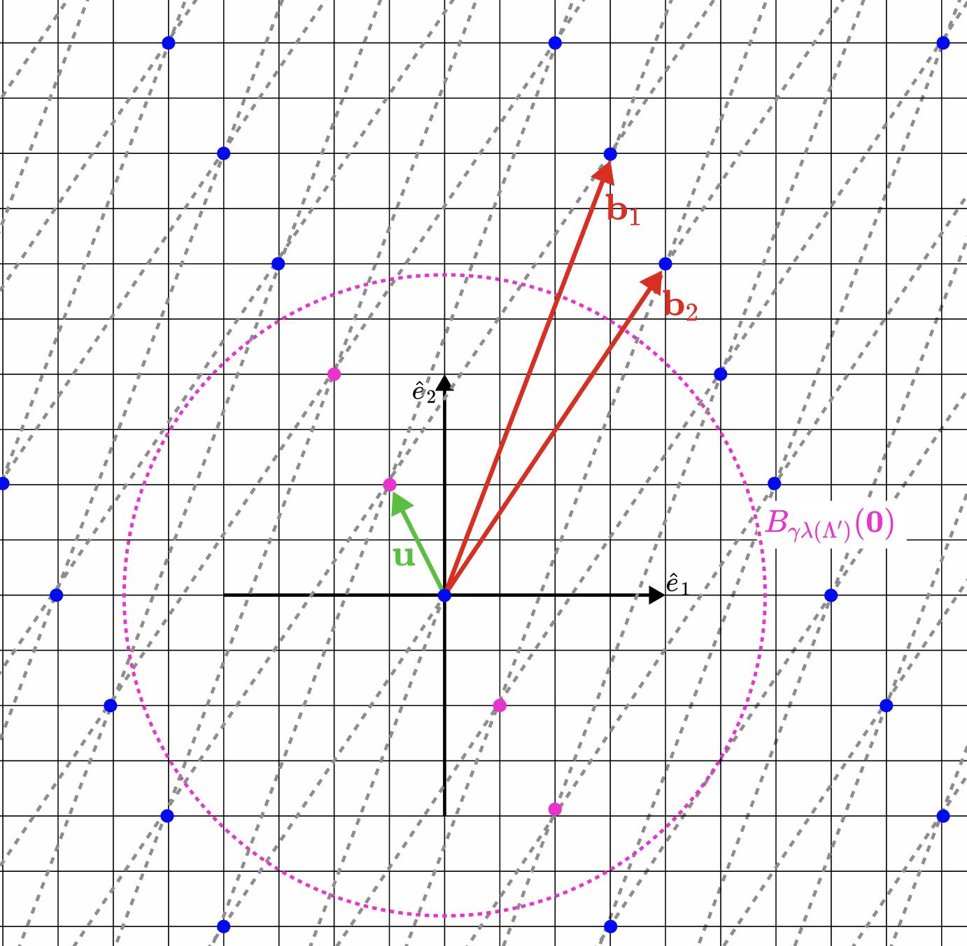
* Figure 2. Explanation of $\gamma$- SVP . Suppose that the lattice $\Lambda'$ is spanned by vectors $\mathbf{b}_1=(3,8)$ and $\mathbf{b}_2=(4,6)$ (incidentally, it is a sublattice of the lattice $\Lambda$ defined in Figure 1 above). Its two shortest vectors are $\mathbf{u}=(-1,2)$ and $-\mathbf{u}$, both with lengths $\lambda_1(\Lambda')=\sqrt{5}$. In this approximate version of $\gamma$ -SVP , $\gamma$ is approximately equal to 2.61 , so we only need to find vectors with lengths shorter than $\sqrt{34}$ (these ranges are marked with purple circles in the figure). For example, the length of $\mathbf{u}'=(2,-4)$ is $\sqrt{20}$. This is the solution for the approximate SVP , but not the solution for the standard SVP .
short integer solutions
While cryptosystems can be constructed directly based on the lattice hypothesis (as Hawk did), in general we use an alternative hypothesis (which can be reduced to the lattice hypothesis). The most famous examples are " Short Integer Solutions ( SIS )" and " Learning with Errors ( LWE )". For the purposes of this article, we will only discuss the former.
Suppose we have a linear equation $\mathbf{Ax}=0$, where $\mathbf{A} \in \mathbb{Z} q^{n \times m}$ ($A$ is an integer matrix of size $n \times m$). Finding the solution to this equation is easy (e.g., through Gaussian elimination). However, suppose we also require that the solution to $\mathbf{x} \in \mathbb{Z}^m$ be "short", i.e., $|\mathbf{x}| {\infty} < \beta$ (where $|\mathbf{x}| {\infty} := \min {i \in [m]}|x_i|$ is the $\ell^{\infty}$ norm of $\mathbf{x}$), and $\beta \ll q$. This becomes an instance of the short integer solution problem, denoted as $\mathsf{SIS}_{q,n,m,\beta}$; and, under carefully chosen $q,n,m,\beta$, it is extremely difficult even for quantum computers.
(Translator's note: For some reason, the definition of the $\ell^{\infty}$ norm used by the author here seems to differ from the common definition, which takes the maximum value of the elements, thus requiring that the short integer solution is that the value of the vector in any dimension is less than $\beta$.)
Exercise 1. Prove that as long as $m>\frac{n\log q}{\log(1+\beta)}$, $\mathsf{SIS}_{q,n,m,\beta}$ has a solution.
Furthermore, we use $S_{\eta}$ to denote the set of "short" vectors, that is:
$$
\begin{equation*}
S_{\eta} := {\mathbf{x} \in \mathbb{Z}^n: |\mathbf{x}|_{\infty} \leq \eta}.
\end{equation*}
$$
Non-homogeneous SIS
A key tweak to this assumption is considering a non-homogeneous version of the same equation: $\mathbf{Ax}=\mathbf{t}$. This modification allows us to consider deterministic hypotheses rather than search hypotheses. Specifically, we introduce the " Nonhomogeneous Short Integer Solutions ( ISSIS )" hypothesis, claiming that distinguishing between the following two distributions $D_0$ and $D_1$ is a computationally difficult problem:
- $D_0$: A sample is randomly selected from $\mathbb{Z}_q^{n \times m} \times \mathbb{Z}_q^n$.
- $D_1$: Randomly sample $A \gets_R \mathbb{Z} q^{n \times m}$, sample a short vector $\mathbf{s} \in \mathbb{Z}^m$ (i.e., $|\mathbf{s}| {\infty} < \delta$), calculate $\mathbf{t} \gets \mathbf{As}$, and then output the tuple $(\mathbf{A}, \mathbf{t})$.
We can prove that ISIS is equivalent to SIS when the underlying $\beta$ and $\delta$ have a proper association. This assumption allows us to develop the following key generation method:
- The private key is a matrix $\mathbf{S} \in S_{\eta}^{m \times k}$, consisting of short elements.
- The public key is $\mathbf{T} := \mathbf{AS}$, where $\mathbf{A} \in \mathbb{Z}_q^{n \times m}$ is randomly sampled.
Exercise 2. Prove that the problem of recovering a private key from a public key is equivalent to solving ISIS (assuming $k = \mathsf{poly}(n)$).
Relationship with case
You might be thinking: What about the lattice? What does this have to do with lattices? One explanation that fits into this blog post is: for instances of $\mathsf{SIS}_{q,n,m,\beta}$ of matrix $\mathbf{A}$, a lattice can be defined as follows:
$$
\begin{equation*}
\Lambda_A^{\perp} = {\mathbf{z} \in \mathbb{Z}^m: \mathbf{Az} = 0 ; (\text{mod} ; q)}.
\end{equation*}
$$
Insight : Solving $\mathsf{SIS}_{q,n,m,\beta}$ is equivalent to solving $\gamma$ -SVP under proper $\gamma$. This can be seen from the definition of $\Lambda_A^{\perp}$: any vector in this lattice is a solution to $\mathbf{A}\mathbf{x}=0$; if we want to solve for the SVP of this lattice, we are essentially looking for short integer solutions to this equation, which is exactly what SIS requires.
Fiat-Shamir Transform with Abort
motivation
We have seen that the lattice-based assumption allows us to construct a one-way mapping $\mathbf{S} \mapsto \mathbf{AS}$ for a given matrix $\mathbf{A}$ and a “short” matrix $\mathbf{S}$. This is somewhat analogous to the mapping $s \mapsto a^s$ being one-way in a cyclic group $\mathbb{G}=\langle a \rangle$, provided the discrete logarithm assumption holds. This leads us to ask the following question:
Can we "recreate" the Schnorr signature protocol by replacing the group multiplication mapping $s \mapsto a^s$ with $\mathbf{S} \mapsto \mathbf{A}\mathbf{S}$?
It can be proven that the answer is yes! However, it's not as simple as it seems, which is the origin of the prefix "with termination". In this section, we'll see how to make this idea a reality.
Schnorr signature scheme
Without further ado, let's review how Schnorr signatures work. Describing a signature scheme means defining the following three procedures:
- $\mathsf{KeyGen}(1^{\lambda}) \to (\mathsf{pk}, \mathsf{sk})$ : Generate a key pair;
- $\mathsf{Sign}(\mathsf{sk},\mu) \to \mathsf{sig}$: Sign the message $\mu$ using the private key sk , thereby generating the signature sig ;
- $\mathsf{Verify}(\mathsf{pk},\mu,\mathsf{sig}) \to {0,1}$: Verify the signature sig based on the public key pk and the message $\mu$.
Schnorr signatures are arguably the most elegant, efficient, and simple signature scheme based on the discrete logarithm assumption, and are now actively used in Bitcoin. However, it's best to start with the Schnorr authentication protocol . Specifically, suppose there is a group of order q $\mathbb{G}$, generated by $g \in \mathbb{G}$; then, to prove that the signer knows the private key $\alpha$ corresponding to the public key $h \in \mathbb{G}$ (where $g^{\alpha}=h$), he participates in the following interactive protocol:

* Figure 3. Schnorr identity recognition protocol, based on key pair $(\alpha,h)$ ( where $h=g^{\alpha}$*)
(Translator's note: The interaction process is as follows: the signer takes a random number r and sends its corresponding value a in the group to the verifier; the verifier takes a random number e and sends it to the signer; the signer uses r, e, and the private key to calculate z and gives it to the verifier.)
The Fiat-Shamir transformation allows signers to avoid interacting with verifiers by deriving $e$ using the hash function $\mathsf{H}: \mathbb{G}^2 \to \mathbb{Z}_q$. Specifically, the signer calculates the challenge value $e \gets \mathsf{H}(h,a)$, which generates the "evidence" $(e,z)$. Finally, to develop a signature scheme , the message $\mu$ can also be included in the derivation of the challenge value $e$. Therefore, $\mathsf{Sign}(h,\mu)$ looks like this:
- Construct a commitment $g^r$ for the random masking scalar $r \gets_R \mathbb{Z}_q$, similar to the identity recognition protocol above;
- Calculate the challenge value: $e \gets \mathsf{H}(\mu,a)$ ;
- Compute the scalar $z = r + \alpha e$, which masks the underlying secret value $\alpha$; output $(e, z)$ as a signature.
Finally, the verifier checks the signature $(h,\mu,\sigma)$ by $e=_?\mathsf{H}(\mu, g^zh^{-e})$.
Attempt #1: Schnorr signature with the character "格"
Since we have found that $\mathbf{S} \mapsto \mathbf{AS}$ looks very similar to the pre-quantum class $\alpha \mapsto g^{\alpha}$, let's try directly putting this one-way mapping into the Schnorr identity recognition protocol, as shown in Figure 4. Following the previously mentioned line of thought, this attempt is a natural first step (we solidify r , a , and e so that matrix multiplication becomes meaningful):
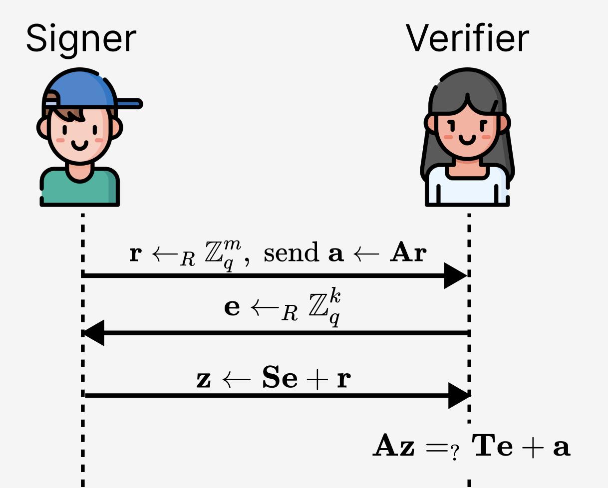
Figure 4. The first attempt at the “grid” Schnorr identity recognition protocol, with the key pair being $(\mathbf{S},\mathbf{T})$ ($\mathbf{T}=\mathbf{AS}$, where $\mathbf{T} \in \mathbb{Z}_q^{n \times k}$, $\mathbf{A} \in \mathbb{Z}_q^{n \times m}$, and $\mathbf{S} \in \mathbb{Z}_q^{m \times k}$).
First, is this scheme formally correct? Let's substitute everything into the verification equation and see:
$$
\begin{equation*}
\mathbf{Az} = \mathbf{A}(\mathbf{S}\mathbf{e}+\mathbf{r}) = (\mathbf{AS})\mathbf{e}+(\mathbf{A}\mathbf{r}) = \mathbf{Te}+\mathbf{a}.
\end{equation*}
$$
Therefore, this plan is formally correct. But is it reliable? Absolutely not. You can find many ways this plan might fail. For example:
- Given $\mathbf{a} \in \mathbb{Z}_q$, it is easy to find r from the commitment equation $\mathbf{a}=\mathbf{Ar}$. In fact, this is simply solving a linear equation on $\mathbb{Z}_q$.
- Even assuming the commitment 'a' is bound, it is possible to find a 'z' that satisfies the equation $\mathbf{Az}=\mathbf{Te}+\mathbf{a}$, even without knowing the private key S. Again, this simply involves solving a linear equation after obtaining any ' e' .
It seems we're stuck at this point.
Try #2: Shrink everything
Note that "Attempt #1" is unsafe because we can easily forge z and easily retrieve a from r . This is because they are simply arbitrary solutions to the system corresponding to these linear equations. As we saw in the SIS hypothesis, we need both z and r to be "short" to fix the reliability of this protocol. Therefore, this attempt aims to achieve this. We will randomly sample r from some short distributions $\chi^m$ (imagine there are some probability distributions $\chi$ on $\mathbb{Z} q$ from which the norm of a sampled value is restricted to a small $\varepsilon \in \mathbb{Z} {>0}$). Making z (and $\mathbf{r}+\mathbf{Se}$) shorter is more difficult: although r is now short, we also need to ensure that Se is short. As a result, because S is already a small value, we need to ensure that e is both short and has a sufficiently large set of possible values. Specifically, we will sample from the set $B_{\kappa}$:
$$
\begin{equation*}
B_{\kappa} := {\mathbf{x} \in \mathbb{Z}_q^k: x_i \in {0,\pm 1} ; \text{and the number of non-zero $x_i$ is $\kappa$}}.
\end{equation*}
$$
To be honest, this set appeared out of thin air (like many things in lattice-based cryptography). The rationale for using this set is probably as follows:
- We want the set of challenge values to be large enough; this set satisfies this condition (see Exercise 3 below);
- We want all elements in this set of challenge values to be small enough; this obviously also holds true, because for every $\mathbf{e} \in B_{\kappa}$, we have $|\mathbf{e}|_{\infty}=1$;
- Ideally, we want the implementation of hashing to $B_{\kappa}$ to be as simple as possible: this also holds true because the elements in $B_{\kappa}$ can be viewed as a ternary string.
Exercise 3. Prove two properties of the set of challenge values $B_{\kappa}$: (a) $#B_{\kappa}=2^{\kappa}\binom{k}{\kappa}$ (i.e., this set is very large); (b) for any $\mathbf{S} \in S_{\eta}^{m \times k}$, we have $|\mathbf{Se}|_{2} \leq \eta\kappa\sqrt{m}$, where $|\cdot|_2$ denotes the standard Euclidean norm (i.e., we have a good boundary for the norm value of Se that is to be included in the computation of z ).
Now, since e and r are both short, z is also short. Therefore, to prevent the adversary from sending large e and r , we need to check that $|\mathbf{z}| 2$ is small enough (i.e., less than a certain threshold $\tau$; you can understand this as $\tau:=\max {\mathbf{e} \in B_{\kappa}}|\mathbf{Se}| 2 + \mathbb{E} {\mathbf{r} \sim \chi^m}[|\mathbf{r}|_2]$, but this is irrelevant to our current level of discussion).
With these modifications, our second attempt looked like this:
Figure 5. The second attempt at the “grid” Schnorr identity recognition protocol, with the key pair $(\mathbf{S},\mathbf{T})$ ($\mathbf{T}=\mathbf{AS}$, where $\mathbf{T} \in \mathbb{Z}_q^{n \times k}$, $\mathbf{A} \in \mathbb{Z}_q^{n \times m}$ and $\mathbf{S} \in \mathbb{Z}_q^{m \times k}$).
Is this solution correct? Yes, for the same reason as "Try #1".
Is it reliable? Hmm, let's look at some "simple" attacks:
- Can we find a shorter r such that $\mathbf{Ar}=\mathbf{a}$? This is equivalent to solving ISIS, and therefore seems computationally infeasible.
- Can we find a shorter z such that $\mathbf{Az}=\mathbf{Te}+\mathbf{a}$? (That is, without knowing S ) Again, this is an example of the ISIS problem, which is also difficult to solve.
So... can we now say that this plan is reliable?
no! :- (
However, the reasoning is quite subtle and becomes easier to discover during the proof of security. Here's a simplified explanation: to recap, the entire purpose of calculating z is to "conceal" the secret value S behind it. But can we say that z and S are independent of each other? Not necessarily.
Note:
If you're trying to recall the security proof of Schnorr signatures, the following explanation might be more helpful: Recall that the proof of EUF-CMA (existence unforgeability under chosen-plaintext attack) consists of two parts: (a) simulating an honest signer; and (b) using a "forking lemma" to extract the secret value behind it. In Figure 5 , it's completely unclear how to perform (a): specifically, where to sample z . Even if we know the distribution of z , it might depend on S , which would cause problems in the simulation.
For this reason, we need to make z and S independent. But how do we do that? It can be proven that the following idea will be useful:
When generating a candidate pair $(\mathbf{e},\mathbf{z})$, first check if the obtained z is "good enough". If not, discard it and repeat the signing process.
This is why this paradigm is called "rejection sampling" or "Fiat-Shamir transformation with abort ": if we are not satisfied with the generated values, we abort the signature process. But what constitutes "good enough" for z ? To do this, we choose a specific distribution $\chi$ that produces some useful properties, and then see when the statistical distance between z and S is negligible.
Discrete Gaussian distribution
If you think the choice of the challenge value space $B_{\kappa}$ is arbitrary, then I would say that this is exactly what I thought was completely arbitrary when I first started learning about lattice-based electronic signatures. Introduce a Gaussian distribution $\Lambda \subseteq \mathbb{R}^m$ on the lattice $\Lambda \subseteq \mathbb{R}^m$, with a width parameter (standard deviation) of $\sigma \in \mathbb{R} {>0}$ and a mean of $\mathbf{v} \in \mathbb{R}^m$, as follows:
$$
\begin{equation*}
D {\mathbf{v},\sigma,\Lambda}^m(\mathbf{z}) := \rho_{\mathbf{v},\sigma}^m(\mathbf{z})/\rho_{\mathbf{v},\sigma}^m(\Lambda) ; \text{where} ; \rho_{\mathbf{v},\sigma}^m(\mathbf{z}) := \exp(-|\mathbf{z}-\mathbf{v}|_2^2/2\sigma^2).
\end{equation*}
$$
(Translator's note: "Gaussian distribution" is the same as "normal distribution".)
Here, we will misuse notation, using $\rho_{\sigma}^m(\Omega)=\sum_{\mathbf{w} \in \Omega}\rho_{\sigma}^m(\mathbf{w})$ to represent the distribution on a discrete set $\Omega \subseteq \mathbb{R}^m$. We omit $\Lambda$ and $\mathbf{v}$ in the index when they are $\Lambda=\mathbb{Z}^m$ and $\mathbf{v}=0$, respectively.
This definition likely requires some explanation. The key idea here is that we want the probability of each point z appearing on the lattice $\Lambda$ to be proportional to $\exp(-|\mathbf{z}-\mathbf{v}| 2^2/2\sigma^2)$. To transform this into an efficient probability distribution, we need to divide all probabilities by a normalization constant $\sum {\mathbf{w} \in \Lambda}\exp(-|\mathbf{w}-\mathbf{v}|_2^2/2\sigma^2)$.
In principle, it is named " Discrete Gaussian Distribution" precisely because it is very similar to the continuous Gaussian distribution (their density is $e^{-|\mathbf{z}-\mathbf{v}|^2/2\sigma^2}/\int_{\mathbb{R}^m}e^{-|\mathbf{z}-\mathbf{v}|^2/2\sigma^2}\text{d}\mathbf{z}$; in the continuous distribution, the integral in the denominator is easy to calculate). Furthermore, if you have seen the shape of this distribution, you will immediately recognize it as a standard multivariate Gaussian distribution:
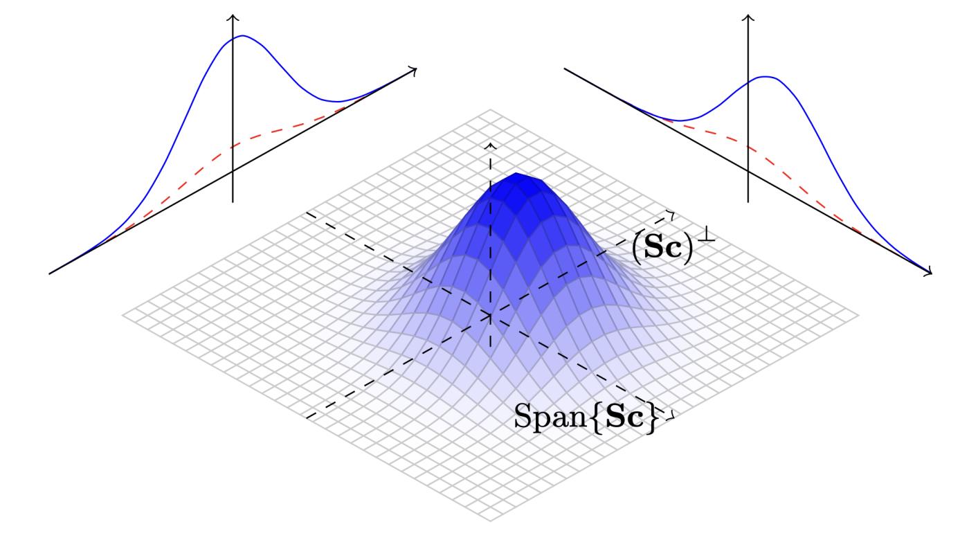
Figure 6. 2D discrete Gaussian distribution. Image from the paper " Lattice Signatures and Bimodal Gaussians " by Ducas, Durmus, Lepoint, and Lyubashevsky.
Why use the discrete Gaussian distribution?
I think the answer to "why choose this specific distribution" is similar to asking why a continuous Gaussian distribution is used in statistics. It's a natural choice because it has good properties under a variety of operations (e.g., it can perform Fourier transforms and convolutions; the sum of discrete Gaussian distributions is statistically close to a single discrete Gaussian distribution, etc.).
However, in our problem (making z and S probabilistically independent), we need two properties of the discrete Gaussian distribution.
Attribute (A) ( The probability of sampling a short vector from $D_{\sigma}^m$ is overwhelmingly high ). For any $\beta>1$, we have:
$$
\begin{equation*}
\text{Pr}[|\mathbf{z}| 2>\beta\sigma\sqrt{m} ; | ; \mathbf{z} \gets_R D {\sigma}^m] < \beta^me^{m(1-\beta^2)/2}.
\end{equation*}
$$
* Property (B) ( The ratio of a central Gaussian distribution to a non-central Gaussian distribution is almost always bounded*) For any $\mathbf{v} \in \mathbb{Z}^m$, as long as $\sigma=\alpha|\mathbf{v}|$, we have:
$$
\begin{equation }
\text{Pr}[D_{\sigma}^m(\mathbf{z})/D_{\mathbf{v},\sigma}^m(\mathbf{z}) < e^{12/\alpha+1/(2\alpha^2)} ; | ; \mathbf{z} \gets_R D_{\sigma}^m] > 1 - 2^{-100}.
\end{equation }
$$
The proofs for both properties require a significant amount of mathematics. See, for example, Chapter 4 of Lyubashevsky's original paper . We will further denote this "magic" constant $e^{12/\alpha+1/(2\alpha^2)}$ as $M_{\alpha}$.
Exercise 4. Assume $\alpha>1$, what is the possible range of $M_{\alpha}$?
While I think property (A) is intuitive (we'll be using it on $\beta$ slightly above 1.0), you might still be wondering why we need property (B) ? The next section will explain that.
Reject sampling
Now, let's assume $\chi^m := D_{\sigma}^m$ in Figure 6. How exactly is z distributed? Because $\mathbf{z}=\mathbf{Se}+\mathbf{r}$, and $\mathbf{r} \sim D_{\sigma}^m$ is a centrally discrete Gaussian distribution, z will be a "biased" Gaussian distribution $D_{\mathbf{Se},\sigma}^m$ with a small offset vector of Se .
This is where the traditional character comes in: The distribution of z depends on a small offset Se ; therefore, by observing multiple z using the same S , an adversary may be able to obtain information about S.
If only we could eliminate this offset... Then the following lemma comes to the rescue:
Lemma. Let $f$ and $g$ be two probability distributions, with the set of all possible values (support) denoted by $\Omega$. For all $\mathbb{R}_{\geq 1}$, $f(z) \leq Mg(z)$. Then, the following distribution (called $\widetilde{f}$) is the same as distribution $f$:
- Random sampling $z \gets_R g$ .
- Output $z$ with probability $f(z)/Mg(z)$, otherwise return to step 1.
Basically, the idea behind this lemma is that if $f$ is our “target distribution” and $g$ is the “true distribution”, then as long as there is a good inequality between points in $f$ and $g$, we can model the distribution of $f$ by discarding some samples from $g$ with probabilities independent of the sampled values.
This process has a good visual representation as shown below (same as Figure 7 , taken from the BLISS paper, a truly excellent illustration). Assume that $f$ and $g$ satisfy the inequality in the lemma, then $Mg$ will be higher than $f$. Then, rejection sampling is formed in two steps: first, select a point from $Mg$; then, if it is lower than $f$, accept it.
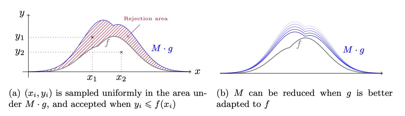
Figure 7. Demonstration of the rejection sampling process. Image taken from the paper " Lattice Signatures and Bimodal Gaussians " by Ducas, Durmus, Lepoint, and Lyubashevsky.
Does this lemma remind you of anything? The key technique is to apply this lemma as follows:
- Our target distribution $f$ is an unbiased discrete Gaussian distribution $D_{\sigma}^m$.
- Our “true” distribution $g$ is a biased Gaussian distribution $D_{\mathbf{Se},\sigma}^m$.
Can we apply this lemma? Property (B) is the key: we have a magic constant $M_{\alpha}$ such that $D_{\sigma}^m(\mathbf{z}) \leq M_{\alpha}D_{\mathbf{Se},\sigma}^m$ holds with overwhelming probability! (Moreover, we can easily confirm $\alpha$ from the fact that $|\mathbf{Se}|_2 \leq \eta\kappa\sqrt{m}$: see Exercise 3 ).
warn
Better safe than sorry, the lemma must be adjusted so that the inequality $f(z) \leq Mg(z)$ occurs with an overwhelming probability of $1-\varepsilon$. Then we can prove that, in this case, the statistical distance between the distribution $\widetilde{f}$ and the distribution $f$ will be $\varepsilon/M$.
Attempt #3: Lyubashevsky's signature
Finally, to fix the solution in Figure 2 , we only accept $(\mathbf{e},\mathbf{z})$ with probability $D_{\sigma}^m(\mathbf{z})/M_{\alpha}D_{\mathbf{Se},\sigma}(\mathbf{z})$. This fixes the entire solution, as shown in the figure below.
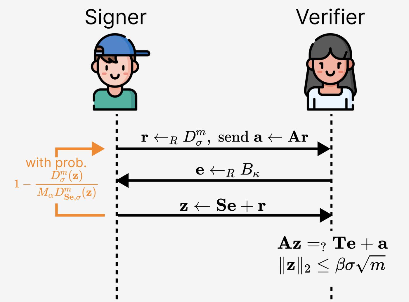
Figure 8. Repairing the lattice-based Schnorr protocol (which is essentially an original solution from the Lyubashevsky paper).
Safety certification skeleton*
Note:
The following section is optional.
To recap, in order to prove that a signature scheme is secure, we need to (a) simulate an honest signer; and (b) use the bifurcation lemma to extract solutions to instances of some computationally difficult problems.
Step (a) is a simple application of the rejection sampling lemma: instead of directly sampling $\mathbf{r} \gets_R D_{\sigma}^m$, calculating the challenge value $\mathbf{e} \gets \mathsf{H}(A\mathbf{r}, \mu) \in B_{\kappa}$, and outputting the candidate $(\mathbf{e}, \mathbf{z}:=\mathbf{Se}+\mathbf{r})$, we first sample $\mathbf{z} \gets_R D_{\sigma}^m$ and $\mathbf{e} \gets_R B_{\kappa}$, and reprogram the random oracle to $\mathsf{H}(\mathbf{Az}-\mathbf{Te},\mu) \gets \mathbf{e}$ .
Step (b) assumes that the adversary can output a valid signature $(\mathbf{z},\mathbf{e})$ with a non-negligible probability $\delta$. According to the bifurcation lemma, TA can output another valid signature $(\mathbf{z}^*,\mathbf{e}^*)$ with a probability $\propto \delta^2$. Furthermore, the underlying randomness is the same, i.e.:
$$
\begin{equation*}
\mathbf{Az} - \mathbf{Te} = \mathbf{Az}^*-\mathbf{Te}^*.
\end{equation*}
$$
Using the fact $\mathbf{T}=\mathbf{AS}$, we can obtain
$$
\begin{equation*}
\mathbf{A}((\mathbf{z}-\mathbf{z}^*)+\mathbf{S}(\mathbf{e}^*-\mathbf{e})) = 0,
\end{equation*}
$$
Here, $(\mathbf{z}-\mathbf{z}^*)+\mathbf{S}(\mathbf{e}^*-\mathbf{e})$ is a short solution to the linear equation $\mathbf{Ax}=0$. Therefore, we construct a reduction that interprets the signature as solving an approximate SIS instance.
performance
Frankly, the aforementioned scheme is very inefficient. Under the parameters proposed in the original paper, the signature size is 19.9KB, while the public key size is 128KB. However, the idea presented above can be optimized in many ways. In particular:
Almost all signatures do not use $\mathbb{Z}_q$, but instead use the ring $\mathcal{R}_q := \mathbb{Z}_q[X]/(X^d+1)$, where $d$ is a power of 2. The reasons why this ring is efficient are beyond the scope of this article.
A distribution other than the discrete Gaussian distribution can be chosen. For example, the BLISS signature scheme proposes a bimodal Gaussian distribution, while other aspects are almost identical to the above construction. The resulting signature size is 5.6KB, and the public key size is 7KB. Unfortunately, this scheme has been proven insecure against side-channel attacks.
If we change the discrete Gaussian distribution to a uniform distribution, we get the Dilithium scheme. However, it is expected that the rejection sampling approach will be quite different (in a sense, simplified).
Next step
In this paper, we analyze a key paradigm of lattice-based electronic signature schemes: the Fiat-Shamir transformation with abort. While it appears in many constructs (and is implicitly used in most papers), there is another paradigm called " hash-and- sign," which is a prerequisite for understanding Falcon and Hawk . These schemes directly utilize lattices and contracts: first, the message $\mu$ is hashed into a point on $\mathbb{Z}^{2n}$, and then this point is transformed using some secret geometric features of the lattice (in Hawk , the private key is the short basis vector B of the specific lattice, and the public key is its square form $\mathbf{B}^{\top}\mathbf{B}$; in Falcon, the public key is the basis of the lattice, and the private key is the basis of its orthogonal lattice).
These directions continue to attract attention from both academia and industry, and for good reason. We are actively exploring these ideas, and future blog posts will return to them.
(over)