
The Glamsterdam equation
Big thanks to @potuz for feedback on the models. Thanks also to @barnabe and @terence.
Overview
The Glamsterdam equation is intended as a guide to the decision between delayed execution and ePBS in the context of shorter slot times. The maximum execution gas/second and blobs/second are computed across both slot pipelining configurations using a set of basic assumptions. A utility maximizing slot configuration is then computed, based on a user’s priorities between scaling, slot time, simplicity, and trustlessness. The Glamsterdam equation should be considered as a tool. It cannot on its own give a definite answer in the debate for two reasons:
- There are several modeling decisions that can bias the outcome in either direction. Certain simplifications were made to produce equations that are easy to overview. Constants were selected by an educated guess and will upon adjustment produce different outcomes.
- We all have different views on the more subjective constants of the utility equation. Subjective qualities such as the value of a trustless exchange or a simple design are not quantified, and the user is simply requested to provide their subjective quantification in U_OUO. They are also able to specify the importance of different scaling components via utility elasticities.
The overall Glamsterdam utility function is specified as
relying on the proportional scaling over Fusaka in gas/s, G^*_s,G∗s, and blobs/s, B^*_s,B∗s, as well as the relative decrease in slot times S^*S∗. Exponents are utility elasticities (default 1) specifying the importance of the different scaling components. The post will first analytically derive the scaling that can be achieved for delayed execution and ePBS respectively across various slot times (following the simplified assumptions), and then return to the utility function. Constants are then varied to analyze the outcome under different assumptions and optimizations. Finally, alternative designs are explored.
Constants
The slot pipelining equations are initially analyzed under the following constants, taking hypothetical Fusaka baselines as a starting point:
| Symbol | Value | Explanation |
|---|---|---|
| L_GLG | 0.8 s | Global latency. The time it takes for a minimal block to propagate sufficiently for consensus formation. |
| L_DLD | 0.8 s/MB | Data latency. The additional time required for full block propagation per MB of data that must be propagated. |
| L_{RF}LRF | 0.2 s | Relay latency. Fixed latency when sending the beacon block to the relay. |
| L_{RD}LRD | 0.15 s/MB | Relay data latency. The additional time required per MB of data when sending the beacon block to the relay. |
| b_bbb | 1 MB | Beacon block size. The maximum size of the beacon block that must be accommodated. |
| P_{bg}Pbg | 1 MB per 60M gas | Payload bytes per gas. The maximum data size of the payload per gas. |
| E_sEs | 60M gas/s | Execution speed. The maximum amount of gas that can be executed per second. |
| B_rBr | 15 blobs/s | Blob rate. The maximum number of blobs that can be propagated per second (derived from 48 blobs/4-L_G4−LG s). |
| \bar{S}¯S | 12 s | Baseline slot length. The baseline Fusaka slot length. |
| \bar{G}_s¯Gs | 5M gas/s | Baseline max gas throughput. The baseline maximum gas/s used as a reference point in the utility function (60M gas/12 s). |
| \bar{B}_s¯Bs | 4 blobs/s | Baseline blob throughput. The baseline blobs/s used as a reference point in the utility function (48 blobs/12 s). |
| A_aAa | 3 s | Attestation aggregation time. The time required for full attestation aggregation. |
| \mathrm{PTC}_dPTCd | 1.4 s | Blob PTC delay. The margin required at the end of the slot fo PTC votes to propagate. |
| A_dAd | 0.4 s | Builder delay. The time a builder waits after the attestation deadline as a worst-case before releasing the payload in ePBS. |
The total relay delay is defined as L_R=L_{RF} + b_\text{b}L_{RD}LR=LRF+bbLRD, with L_RLR used throughout the post instead of writing out individual components.
Constants are educated guesses, based on previous analysis and current developments, e.g.,: 1, 2, 3, 4, 5, 6, 7, 8, 9. The impact of constants with higher uncertainty may sometimes average out to produce realistic outcomes. For example, the data latency L_DLD may be somewhat conservative, whereas the payload bytes per gas P_{bg}Pbg is on the aggressive side, presuming some further adjustments to data costs. To help the reader form their individual opinion:
- the source code for running the analysis and making the plots will be made available online (this weekend),
- the concluding sections explore variations on the baseline settings.
One specific simplification of the analysis that can be highlighted is that the interaction between blob and block propagation at the p2p layer is not modeled, whereas the interaction between beacon block and payload propagation is. The number of blobs per slot is simply derived from available propagation time (which depends on the slot structure) anchored at the Fusaka specification, including the same global delay L_GLG as also applied for blocks. This makes the analysis more tractable. It is also an open question exactly how blobs interact with blocks, given various validator roles and the CL/EL interaction.
Delayed execution
Delayed execution uses the simple configuration with no special header deadline and where blobs must be available at attestation time. The goal of the analysis is to set the attestation deadline AA to maximize utility, which is a function of gas and blob throughput. The total gas, GG, that can be included in a slot is constrained by execution and propagation time. The fixed time constraints on payload propagation can be expressed as
consisting of the relay delay and global delay as well as propagation of the beacon block (consuming a fixed amount of bandwidth that cannot at the same time be used for the payload). The maximum payload size for a given amount of gas GG is P_{bg}GPbgG bytes, where P_{bg}Pbg is the maximum payload size per unit of gas. The time to propagate this payload is subject to the available window A-cA−c, which gives the constraint:
Gas is also limited by the execution window, S-AS−A, and the execution speed, E_sEs (gas/s), giving the second constraint:
The deadline that maximizes the potential gas throughput, A_GAG, is found where the two limits on GG are equal:
Solving for A_GAG yields:
However, the overall goal is to maximize utility, which also includes blob throughput. Define the total number of blobs in a slot as BB. The scaling terms of the utility function are defined as the change in gas/s and blobs/s respectively relative to the current baseline (highlighted by bars):
The utility-maximizing deadline A_UAU is found by maximizing the product of the scaling terms of the overall utility function:
A useful assumption is that the sought optimum is execution limited (i.e., G \propto S-AG∝S−A), because a later deadline always improves blob throughput. To find this optimum, the log-utility \ln U_2lnU2 is analyzed. Ignoring constant terms that do not affect the derivative with respect to AA, the function simplifies to:
Taking the derivative with respect to AA gives:
Setting the derivative to zero and solving for AA gives the final expression:
The final optimal deadline, A^*A∗, is then selected by choosing the later of these two candidates, clamped by the latest admissible deadline that allows for attestation aggregation, A_L = S - A_aAL=S−Aa:
Once the final deadline A^*A∗ is chosen, the total absolute gas GG achievable at that deadline can be calculated by taking the minimum of the two limits:
From this, the final throughputs are derived. The gas per second is:
and the blobs per second, determined by the deadline A^*A∗ and the blob propagation rate B_rBr, is:
Figure 1 shows the optimal attestation deadline, which is either:
- perfectly balanced between payload propagation time and execution time (A_GAG; magenta),
- at the utility optimum when ignoring constraints on payload propagation time (A_UAU; red),
- at the latest point that allows for attestation aggregation (A_LAL; purple).
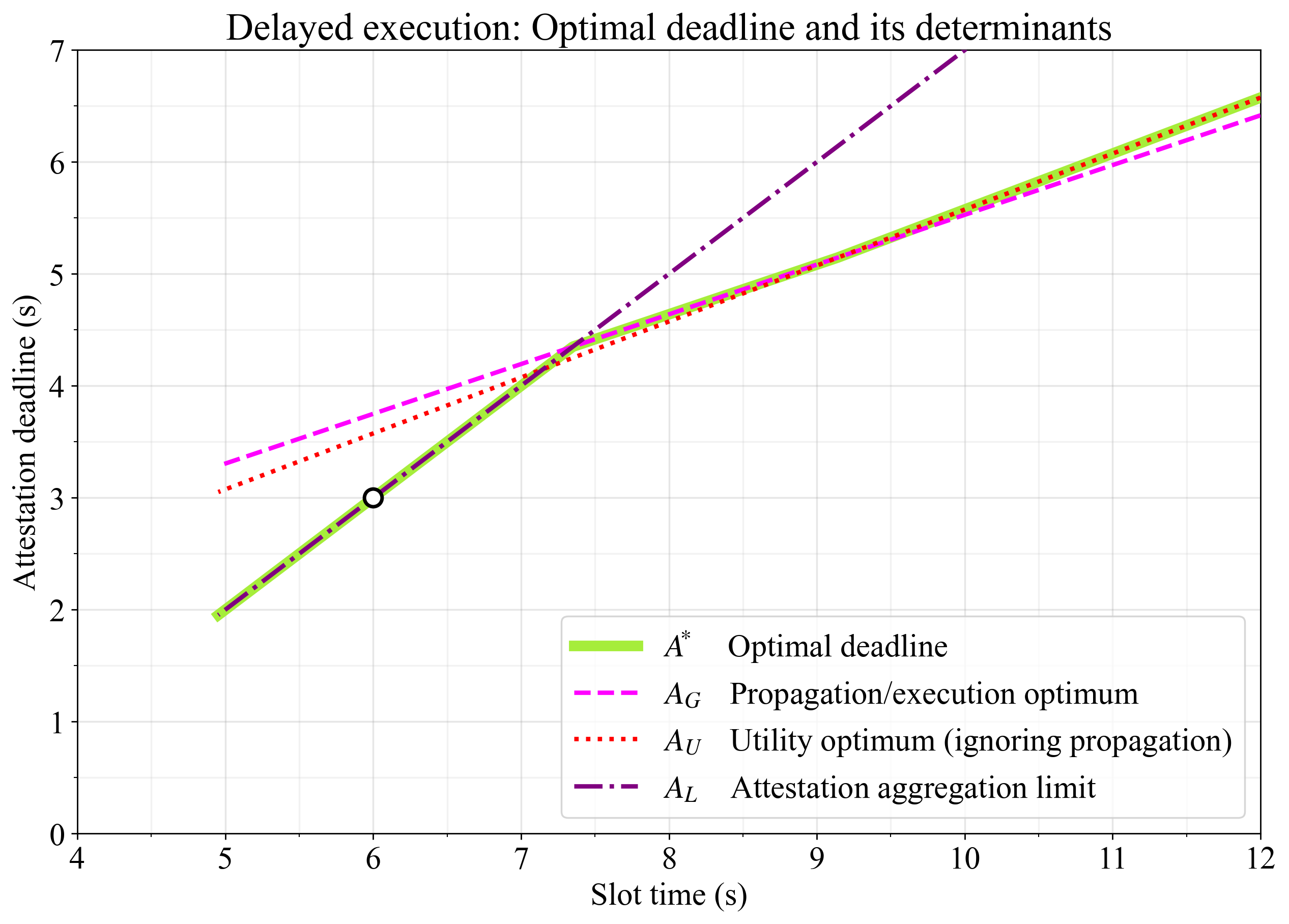
Figure 1. Optimal deadline in delayed execution as the propagation/execution gas optimum A_GAG, the utility maximum in a purely execution-limited model A_UAU, and the latest point that allows for attestation aggregation A_LAL. The circle indicates a potential target at an attestation deadline of 3s in a 6s slot. For optimal throughput, this would require some optimizations to improve propagation time (pushing the optimized lines downward).
With the default constants, the optimal deadline when the slot is 12s long is located at around 6.5s (A_UAU regime). Below slot times of around 9s, payload propagation time constrains the utility optimum for blobs and execution, making it necessary to compromise by selecting a later attestation deadline (A_GAG regime). When the slot time falls below around 7.3s, there is no longer enough time for attestation aggregation under A_GAG, and throughput (propagation) must be compromised by selecting an earlier deadline (A_LAL regime). It is likely that an implementation of delayed execution under 6s slot times would target the circle at a 3s attestation deadline (as has already been proposed). To achieve a high throughput at 6s, it is then necessary to speed up propagation (pushing down optimized lines in Figure 1) through optimizations such as:
- making call data more expensive,
- improving the p2p layer,
- implementing a multidimensional fee market or macro pricing (to bound worst-case payload sizes).
It can also be assumed that builders themselves may select payload compositions that balance propagation and execution for any given deadline, giving leeway to early deadlines. This will however strain payload propagation for payloads with larger bytesizes. Such payloads may be impossible to get accepted even though they adhere to the gaslimit. This is one of the reasons for why a multidimensional fee market is so attractive.
ePBS
The dual-deadline approach is used when modeling ePBS, allowing for an optimal payload PTC deadline \mathrm{PTC}_PPTCP while keeping the PTC DA deadline at the latest possible point of the slot
The payload is released in a trustless setting where the builder in the worst case must release the payload A_dAd after the attestation deadline. A discussion of the relevance of including A_dAd in the analysis is offered in Appendix A. The release of blobs is set to cc such that the builder does not wait A_dAd to count attestations before releasing them, allowing slightly longer time for propagation. The attestation deadline is in ePBS set earlier than in delayed execution, specifically at the constant cc:
The payload is then released at c+A_dc+Ad, and inherits its own global latency L_GLG when propagating as well. The only remaining task is to compute the optimal PTC deadline for the payload, \mathrm{PTC}_PPTCP, which is strictly determined as the point that maximizes the total gas, GG.
The amount of gas is limited by the execution window, S-\mathrm{PTC}_PS−PTCP, and the execution speed, E_sEs (gas/s):
It is also limited by the time required to propagate the payload. A payload of gas GG takes up to L_G + (G \cdot P_{bg} \cdot L_D)LG+(G⋅Pbg⋅LD) to propagate, and must be allowed to arrive at the latest at the \mathrm{PTC}_PPTCP deadline:
This gives the gas constraint on propagation:
The optimal deadline \mathrm{PTC}^*_PPTC∗P is found where the two limits on GG are equal:
Solving this for \mathrm{PTC}_PPTCP and clamping by \mathrm{PTC}_BPTCB yields the final equation:
Once the optimal deadline \mathrm{PTC}^*_PPTC∗P is found, the final throughputs can be determined. The gas per second, G_sGs, is derived from the propagation constraint:
The blobs per second, B_sBs, is determined by the time available for blob propagation—from their release at cc until the blob deadline \mathrm{PTC}_BPTCB, also accounting for their own global latency $L_G$—and the blob rate, B_rBr:
Figure 2 shows the optimal deadlines for maximizing throughput in ePBS under the baseline constants.
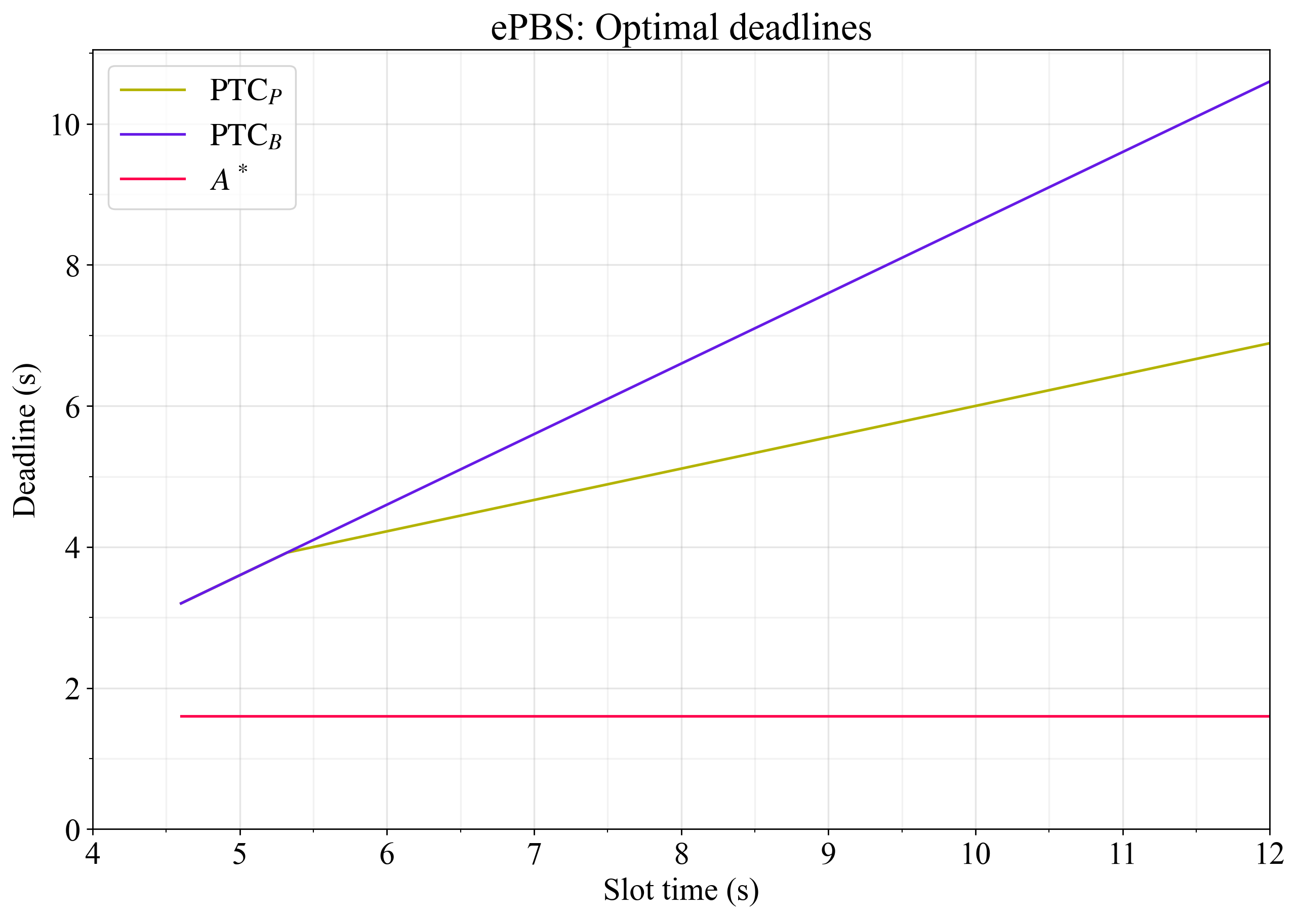
Figure 2. Optimal deadlines for maximizing throughput in ePBS under the baseline constants. The payload observation deadline \mathrm{PTC}^*_PPTC∗P is set at the point that perfectly balances between propagation and execution, adhering to the limit that it cannot happen after the PTC casts its votes at \mathrm{PTC}_BPTCB.
Throughput for delayed execution and ePBS
Figure 3 shows execution Mgas/s and blobs/s for delayed execution and ePBS. As evident, ePBS is particularly suitable for scaling blobs, due to the late PTC deadline that it offers. Since the deadline on the payload can be set independently, there is a smooth decay in throughput as the slot time shortens until propagation finally is constrained below 5.5s. Throughput falls smoothly due to the increasing relative importance of:
- the global delay L_GLG,
- the beacon block propagation time cc,
- the time the builder requires for ascertaining that the beacon block will gather enough attestations A_dAd,
- and the PTC vote propagation time \mathrm{PTC}_dPTCd.
Delayed execution is best for scaling L1 gas at longer slot times, since there is L_G-L_R+A_dLG−LR+Ad less delay incurred at the start of the slot and the attestation deadline can be reasonably well balanced between propagation and execution with the default constants. There is then a kink in the throughput curve as the attestation aggregation constraint comes into play at around 7.3s. Throughput falls substantially below this slot length, due to insufficient time for propagation under the baseline constants.
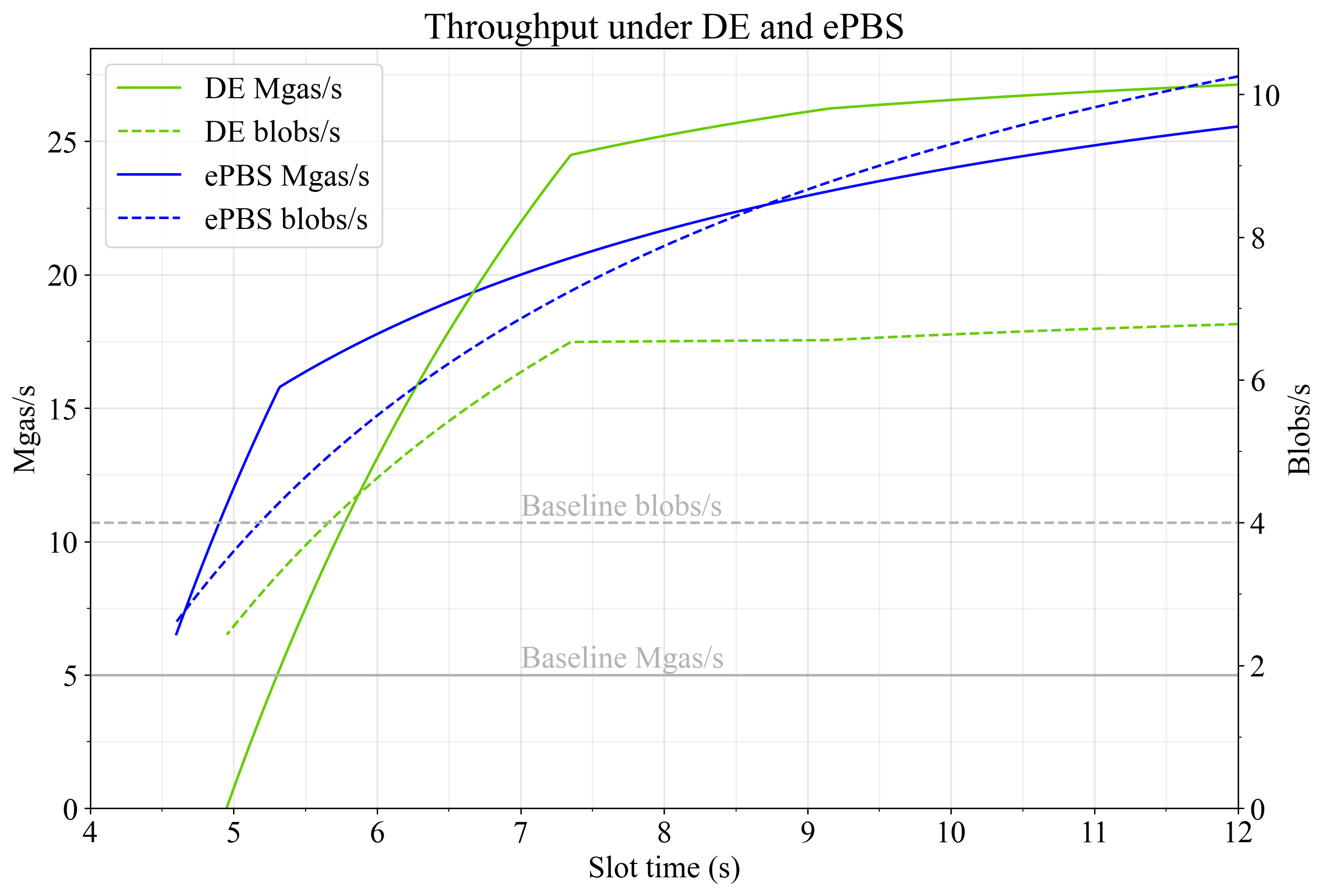
Figure 3. Throughput under delayed execution (green) and ePBS (blue) at different slot times, specified as Mgas/s (full lines) and blobs/s (dashed lines). Both approaches have the potential to scale Ethereum significantly, even at shorter slot times.
Utility according to the Glamsterdam equation
The Glamsterdam equation captures scaling from slot-restructuring, factoring in the relative change in slot time S^*S∗ and a subjective scaling factor U_OUO that captures any additional considerations. Someone may assign U_O>1UO>1 to DE if the simplicity of not changing fork choice and not having a PTC is prioritized. If on the other hand, e.g., a trustless payment between builder and proposer is seen as critical, someone may instead assign U_O>1UO>1 to ePBS. The full equation is:
The equation also features utility elasticities, which specify the importance of different performance metrics in the utility measure. A utility elasticity of 1 indicates that utility is directly proportional to the metric, while an elasticity of 0 indicates that the metric is irrelevant to overall utility. These elasticities are:
- U_GUG – The utility elasticity of execution throughput.
- U_BUB – The utility elasticity of blob throughput.
- U_SUS – The utility elasticity of shorter slot times.
Figure 4 shows how the utility of delayed execution and ePBS changes across slot time, using the settings U_G=1UG=1, U_B=1UB=1, U_S=1US=1, and U_O=1UO=1. Both restructuring options give about equal utility gains, with DE peaking at 7.3s slot times and ePBS at around 10s slot times.
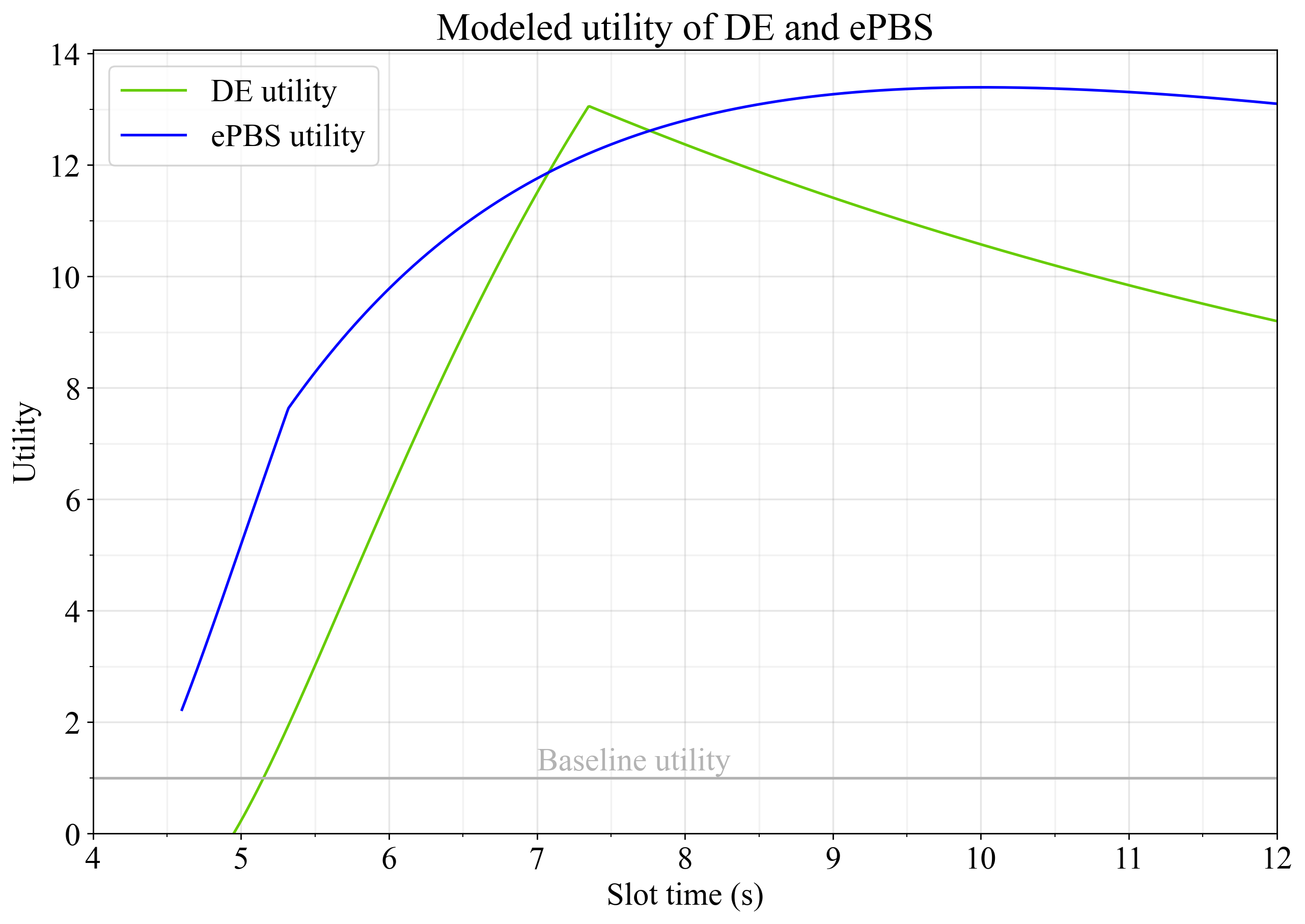
Figure 4. Utility of delayed execution and ePBS when all elasticities are set to 1 and U_O=1UO=1 for both options.
We all have different perspectives on which metrics that are the most important, and the elasticities are then useful. For example, given that a target of 32 blobs per slot already is a significant improvement planned for Fusaka and that the current target of 6 blobs is not actually consumed, it may seem reasonable to assign further scaling of blobs a lower importance than scaling of execution gas. Elasticities of U_G=1UG=1 and U_B=0.4UB=0.4 capture this notion. Shortening slot times might be assigned somewhere in between in terms of importance, for example U_S=0.7US=0.7.
Figure 5 shows the outcome with these elasticities, which somewhat favor delayed execution due to the lower assigned importance of blob scaling. On the other hand, some may perceive ePBS as inherently better, due to its ability to facilitate trustless cooperation between builder and proposer. Setting U_O=1.1UO=1.1 for ePBS captures the notion of ePBS being 10% better than delayed execution in terms of non-measurable qualities. The blue dashed line captures this, and utility is maximized either with ePBS at around 9s slot times, or with DE at 7.3s slot times.
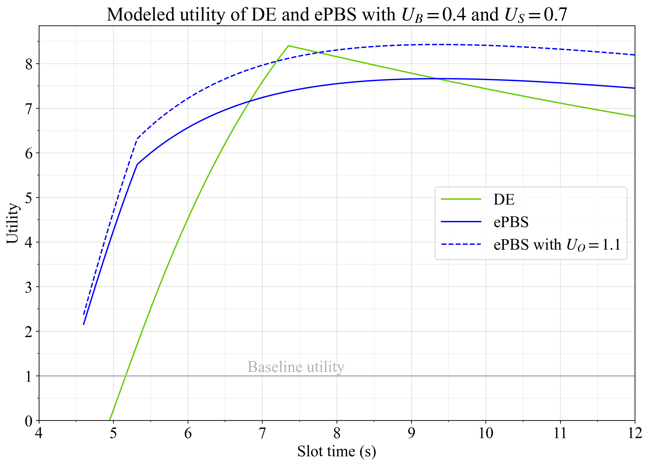
Figure 5. Utility of delayed execution and ePBS with elasticities U_G=1,UG=1, U_B=0.4UB