Preamble
Are you ready to explore a more complex side of zk-SNARK ? In the previous section, we learned about some more advanced concepts such as Arithmetic Circuit and Quadratic Arithmetic Program . In this section, we'll expand our knowledge by delving into another powerful concept: Elliptic Curve Pairings .
Note : Understanding a topic like Elliptic Curve Pairings in depth can sometimes be a challenge for many people. However, that's why we have this article – to help you get at least a basic perspective on this.
My goal is not only to explain Elliptic Curve Pairings thoroughly but also to make the topic more interesting and easy to understand. Hopefully, through this article, you will see the power of elliptic curve pairs in mathematics and cryptography in general, as well as in their specific applications in zk-SNARK in particular.
Elliptic curves
Elliptic curves are part of the field Elliptic Curve Cryptography . This is a complex subject that is not easy for everyone to understand. To understand them better, take a XEM at my article on ECC in the previous section.
Elliptic Curve Cryptography involves “points” in two-dimensional space, each “point” characterized by a pair of (x, y) coordinates.
There are specific rules for performing mathematical operations such as addition and subtraction between points, allowing the coordinates of a new point to be calculated when other points are known.
Example : Calculate coordinates R = P + Q
You can also multiply a point by an integer by repeatedly adding the point to itself as many times as that integer.
For example : P * n = P + P + … + P
This provides an efficient way to perform mathematical operations in Elliptic Curve Cryptography

On an elliptic curve, there is a special point called the “point at infinity” ( O ), equivalent to the number 0 in point calculus, which is always true that P + O = P.
A curve also has an “order” ; There exists a number n such that P * n = O for all P ( P * (n+1) = P, P * (7*n + 5) = P * 5 , and so on).
In addition, there is also a “generator point” (G ), which is understood to represent the number 1 in some way. In theory, any point on the curve (except O ) can be G .
Pairings
Pairings allow testing of more complex equations on points of an elliptic curve.
For example:

you can check XEM p * q is equal to r just from P, Q and R .
Although information about p can leak from P , this leakage is carefully controlled.
Pairings allow checking quadratic constraints .
For example: Testing e(P, Q) * e(G, G * 5) = 1 is actually testing p * q + 5 = 0 .

is an operation called pairing . Mathematicians also call it a bilinear mapping . “Bilinear” here will comply with the following rules:
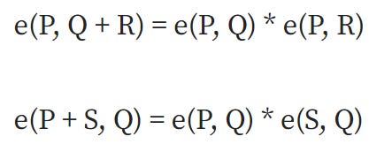
Note that you can use the + and * operators in any way, as long as they comply with the following rules:
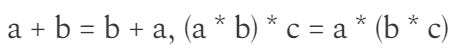
and

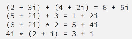
If P, Q, R and S are simple numbers, creating a simple pairing operation is easy with the expression:
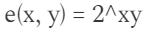
The following results:

That's the parallel line !
However, such simple pairing operations are not suitable for cryptography because they operate on simple integers and are too easy to analyze.
When you know a number and its result when performing the pairing operation, you can easily calculate and find the remaining number.
We use mathematical operations like "black boxes" , where only basic mathematical operations can be performed without further analysis or understanding. This is why elliptic curves and pairing operations on elliptic curves become important in cryptography.
Prime Fields and Extension Fields
It is possible to create a bilinear map on elliptic curve points — that is, create a function

where P and Q are elliptic curve points, and the result is an element type called F_p¹²
First, let's understand prime fields and extension fields.
The Elliptic curve in the image above is so beautiful because the equation of the curve is defined using ordinary real numbers.
However, in Cryptology, using conventional real numbers can lead to using logarithms to “go backwards” , and spoil things as the amount of space required to store and represent numbers can increase arbitrarily. Therefore, we use numbers in a prime fields .
A prime field includes the set of numbers 0, 1, 2… p-1, where p is a prime number and the various operations are defined as follows:

All operations are performed modulo p
Chia is a special case; normally, 3/2 is not an integer, and now I only want to deal with integers, so instead I try to find the number x such that
x * 2 = 3 .
This can be done using Extended Euclidean Algorithm . For example, if p = 7 , then:

Next, we will talk about extension fields .
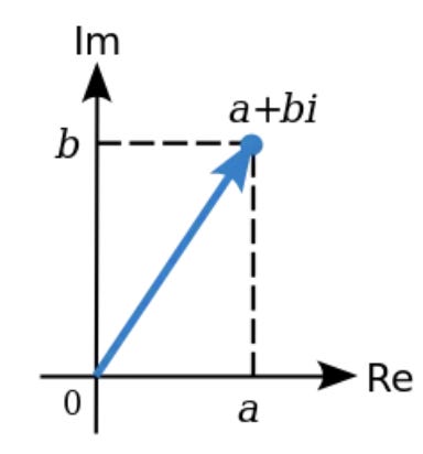
A common example you will often encounter in math books is the complex number field , where the real number field is “ extended ” with the additional element sqrt(-1) = i .
Extension fields work by taking an existing field, then “ adding ” a new element and defining a relationship between that new element and the elements already in the original field (e.g. i² + 1 = 0 ).
The important thing is that this equation is not true for any number in the original field, and then XEM all linear combinations of the elements in the original field and the new element just created.
We can also expand prime fields
For example, extending the prime field mod 7 we described above with i, we can do the following:
If you want to see all the math done in code, prime fields and field extensions are done here
Elliptic Curve Pairings
Elliptic Curve pairing is a mechanism that takes two points from two Elliptic curves and maps those points into a single number.
You can think of this mapping as equivalent to multiplying points on an Elliptic curve.
Mathematically, Elliptic Curve pairing is defined as mapping two points on an Elliptic curve to an element in another group such as a finite field :

Here e is pairing , E 1 and E 2 are Elliptic Curves and 𝐹 is a finite field .

Note that Elliptic Curves E 1 and E 2 need not be different.
Once concatenation occurs, the result is that an element in another group cannot be reused for the next concatenation.
Elliptic Curve Pairings have certain properties called bilinear mappings :

Here P , Q and R are points on the Elliptic Curve and 𝑎∈𝑍, 𝑏∈𝑍
By using these “bilinear mappings” , we can “move around ” the coefficients 𝑎 and 𝑏 on those two curves while keeping the mapping intact:

We can imagine Elliptic curve pairing as a mapping from G2 x G1 -> GT , in which:
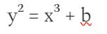
G1 is an elliptic curve, where the points satisfy a form equation
and both coordinates are elements of F_p (they are simple numbers, but the operations are performed modulo a particular prime number)
G2 is also an elliptic curve, where the points satisfy the same equation as G1 , but their coordinates belong to the field F_p¹² (we define a new “ magic number ” w , defined by a polynomial of degree 12 like:

GT is the type of object that the result of the elliptic curve goes into. In the curves we XEM , GT is F_p¹² (the same strong complex number as used in G2 )
Here it must satisfy bilinearity:

Along with two other important criteria:
- Efficient computability: Efficient computing ability means being able to calculate compound operations quickly and without too much complexity. For example : If we simply took the discrete logarithm of the points and multiplied them together to create a compound, this would become computationally too difficult, like breaking the original elliptic curve code. head. Therefore, a compound operation is considered computationally efficient if it can be computed efficiently without imposing too much computational burden.
- Non-degeneracy: Non-degeneracy ensures that the concatenation is not a useless concatenation, i.e. it does not just return a fixed value that is independent of the input points. For example : If we define the coupling as e(P, Q) = 1 for all P and Q , this does not provide any useful information about the relationship between points on the elliptic curve. Therefore, a concatenation is considered Non-degenerative if it provides useful information about the relationship between input points.
So how to do that?
First, we need to understand the concept of divisor , another way to represent functions on points on an elliptic curve.
A divisor of a function essentially counts the zeros and infinity numbers of the function. To understand what this means, let's XEM at some examples. Let's fix some points P = (P_x, P_y) , and XEM the following function:

The divisor is [P] + [-P] – 2 * [O]
[P] + [Q] is not the same as [P + Q]. The reasons are as follows:
- The function is 0 at P because when x is P_x, so x – P_x = 0.
- The function is 0 at -P because -P and P have the same x coordinates.
- The function goes to infinity as x goes to infinity, so we say the function is infinite at O .
The reason is in the equation of the Elliptic curve:

y increases to infinity about “1.5 times” faster than x to keep up with x^3 . Therefore, if a linear function has only x , it will be represented as infinity with a multiple of 2, but if the function has y , then it will be represented as infinity with a multiple of 3.
Now, XEM a “line function” :

Where a, b and c are carefully chosen so that the straight line passes through points P and Q on the Elliptic curve.
Because of the way addition on elliptic curves works, this also means that it passes through the point -PQ . This function also goes to infinity depending on both x and y , thus Chia the possibility of becoming


Each “rational function” (a function defined using only a finite number of operations +, -, *, / on point coordinates) uniquely corresponds to a divsor , with the condition of multiplying by a constant (i.e. if two functions F and G have the same divisor , then F = G * k where k is a constant).
The Chia of the product of two functions is equal to the sum of the Chia of each function, so

then

Article source: Team Tech/Research Alphatrue
Reference source: