In this post we will analyze the consequences that the shape of the issuance curve has for the decentralization of the validator set.
The course of action is the following:
First, we will introduce the concept of effective yield as the yield observed after taking into account the dilution generated by issuance.
Second, we will introduce the concept of real yield as the effective yield that a validator obtains post expenses (OpEx, CapEx, taxes…).
Armed with these definitions we will be able to make some observations about how the shape of the issuance curve can result in centralization forces, as the real yield observed can push out small uncorrelated stakers at high stake rates.
Then, we will propose a number of properties we would expect the issuance curve to satisfy to minimize these centralization forces. And explore some alternative issuance curves that could deal with the aforementioned issues.
Finally, some heuristic arguments on how to fix a specific choice of issuance and yield curves.
Source Code for all plots can be found here: GitHub - pa7x1/ethereum-issuance
Effective Yield
By effective yield we mean the yield observed by an Ethereum holder after taking into account circulating supply changes. For instance, if everyone were to be a staker, the yield observed would be effectively 0%. As the new issuance is split evenly among all participants, the ownership of the circulating supply experienced by each staker would not change. Pre-taxes and other associated costs this situation resembles more a token re-denomination or a fractional stock split. So we would expect the effective yield to progressively reach 0% as stake rates grow to 100%.
On the other hand, non-staking holders are being diluted by the newly minted issuance. This causes holders to experience a negative effective yield due to issuance. We would expect this effect to be more and more acute as stake rates grow closer and closer to 100%.
These ideas can be put very simply in math terms.
Let’s call ss the amount of ETH held by stakers, hh the amount of ETH held by non-stakers (holders), and tt the total circulating supply. Then:
s + h = ts+h=t
After staking for certain period of time, we will reach a new situation s' + h' = t's′+h′=t′. Where s's′ and t't′ have been inflated by the new issuance ii are obviously related to the nominal staking yield y_sys:
s' = s + i = s \cdot y_ss′=s+i=s⋅ys
h' = hh′=h
t' = t + i = t + s \cdot (y_s - 1)t′=t+i=t+s⋅(ys−1)
Now, let’s introduce the normalized quantities s_nsn and h_nhn. They simply represent the proportion of total circulating supply that each subset represents:
s_n \equiv \frac{s}{t}sn≡st
h_n \equiv \frac{h}{t}hn≡ht
We can do the same for s'_ns′n and h'_nh′n:
s'_n \equiv \frac{s'}{t'} = \frac{sy_s}{s(y_s - 1) +t}s′n≡s′t′=syss(ys−1)+t
h'_n \equiv \frac{h'}{t'} = \frac{t-s}{s(y_s - 1) + t}h′n≡h′t′=t−ss(ys−1)+t
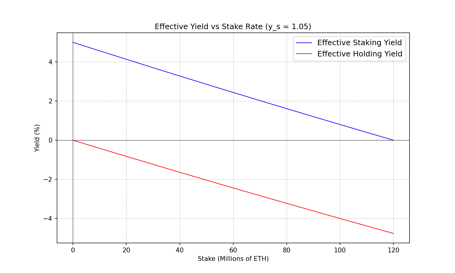
With these definitions we can now introduce the effective yield as the change in the proportion of the total circulating supply observed by each subset.
y_s^{eff} \equiv \frac{s'_n}{s_n} = \frac{y_s}{\frac{s}{t}(y_s-1) + 1}yeffs≡s′nsn=ysst(ys−1)+1
y_h^{eff} \equiv \frac{h'_n}{h_n} = \frac{1}{\frac{s}{t}(y_s-1) + 1} yeffh≡h′nhn=1st(ys−1)+1
Net Yield
Staking has associated costs. A staker must acquire a consumer-grade PC, it must pay some amount (albeit small) for electricity, it must have a high-speed internet connection. And they also must put their own labor and time to maintain the system operational and secure, or must pay someone to do that job for them. Stakers also observe other forms of costs that eat away from the nominal yield they observe, e.g. taxes. We would like to model this net yield observed after all forms of costs, because it can give us valuable information on how different stakers are impacted by changes in the nominal stake yield.
To model this we will introduce two types of costs; costs that scale with the nominal yield (e.g. taxes or fees charged by an LST would fit under this umbrella), and costs that do not (i.e. HW, electricity, internet, labor…).
With our definitions, after staking for a reference period stakers would have earned s' = y_s s = s + s(y_s - 1)s′=yss=s+s(ys−1)
But if we introduce costs that eat away from the nominal yield (let’s call them kk), and costs that eat away from the principal (let’s call them cc). We arrive to the following formula for the net stake:
s' = s(1-c) + s(y_s - 1) - \max(0, sk(y_s - 1))s′=s(1−c)+s(ys−1)−max(0,sk(ys−1))
NOTE: The max simply prevents that a cost that scales with yield becomes a profit if yield goes negative. For instance, if yield goes negative it’s unlikely that an LST will pay the LST holders 10%. Or if yield goes negative you may not be able to recoup in taxes as if it were negative income. In those cases we set it to 0. This will become useful later on when we explore issuance curves with negative issuance regimes.
This represents the net stake our stakers observe after all forms of costs have been taken into account. To be noted that this formula can be easily modified to take into account other types of effects like validator effectiveness (acts as multiplicative factor on the terms (y_s - 1)(ys−1)) or correlation/anti-correlation incentives (which alter y_sys).
To fix ideas, let’s estimate the net yield observed by 3 different types of stakers. A home staker, an LST holder, and an institutional large-scale operator. The values proposed are only orientative and should be tuned to best reflect the realities of each stakeholder.
A home staker will have to pay for a PC that they amortize over 5 years and costs around 1000 USD, so 200 USD/year. Pay for Internet, 50 USD per month, for around 600 USD/year. Something extra for electricity, less than 100 USD/year for a typical NUC. Let’s assume they are a hobbyist and decide to do this with their spare time, valuing their time at 0 USD/year. This would mean that his staking operation has a cost of around 1000 USD/year for them. If they have 32 ETH, with current ETH prices we can round that at ~100K USD. This would mean that for this staker, c = \frac{1}{1000}c=11000. As their costs represent around 1 over 1000 their stake value.
Now for the costs that scale with the yield. They will have to pay taxes, these are highly dependent on their tax jurisdiction, but may vary between 20% and 50% in most developed countries. Let’s pick 35% as an intermediate value. In that case, their stake after costs looks like:
s' = s\left(1-\frac{1}{1000}\right) + s(1-0.35)(y_s - 1)s′=s(1−11000)+s(1−0.35)(ys−1)
We can do the same exercise for a staker using an LST. In this case, c=0c=0 and kk is composed of staking fees (10-15%) and taxes (20-50%) which depend on the tax treatment. Rebasing tokens have the advantage of postponing the realization of capital gains. If we assume a 5 year holding period, equivalent to the amortization time we assumed for solo staking, it could look something like this:
- Fixed costs: 0
- Staking fees: 10%
- Capital gains tax: 20%
- Holding period: 5 years
s' = s(1-0) + s(1-0.14)(y_s - 1)s′=s(1−0)+s(1−0.14)(ys−1)
Finally, for a large scale operator. They have higher fixed costs, they will have to pay for labor, etc… But also will run much higher amount of validators. In that case, c can get much smaller as it’s a proportion of s. Perhaps 1 or 2 orders of magnitude smaller. And taxes will be typical of corporate tax rates (20-30%).
s' = s\left(1-\frac{1}{10000}\right) + s(1-0.25)(y_s - 1)s′=s(1−110000)+s(1−0.25)(ys−1)
Net Effective Yield (a.k.a Real Yield)
Finally, we can blend the two concepts together to understand what’s the real yield a staker or holder obtains net of all forms of costs and after supply changes dilution. I would suggest calling this net effective yield as the real yield, because well, that’s the yield you are really getting.
y_s^{real} = \frac{(1-c) + (y_s - 1) - \max(0,k(y_s - 1))}{\frac{s}{t}(y_s-1)+1}yreals=(1−c)+(ys−1)−max(0,k(ys−1))st(ys−1)+1
y_h^{real} = y_h^{eff} = \frac{1}{\frac{s}{t}(y_s-1) + 1}yrealh=yeffh=1st(ys−1)+1
In the second equation we are simply stating the fact that there is no cost to holding, so the real yield (after costs) of holding is the same as the effective yield of holding.
The Issuance Curve and Centralization
Up to here all the equations presented are agnostic of Ethereum’s specificities and in fact are equally applicable to any other scenario where stakeholders observe a yield but that yield is coming from new issuance.
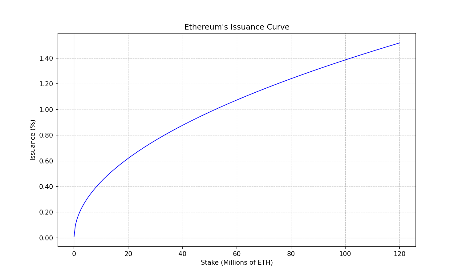
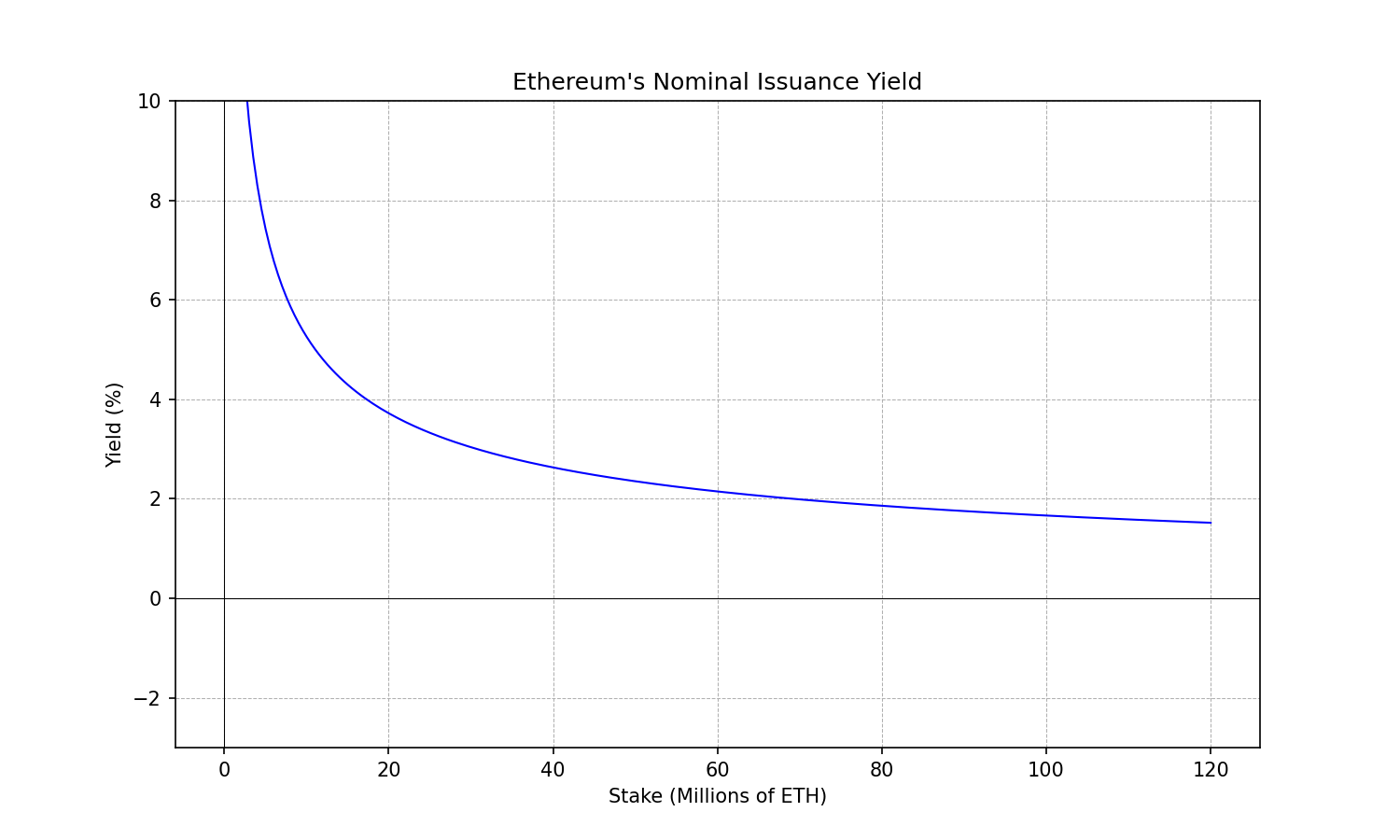
To bring this analysis back to Ethereum-land it suffices to substitute y_sys by Ethereum’s issuance yield as a function of the total amount staked ss. And substitute tt by the total circulating supply of ETH.
t \approx 120\cdot 10^6 \quad \text{ETH}t≈120⋅106ETH
i(s) = 2.6 \cdot 64 \cdot \sqrt{s} \quad \text{ETH}\cdot\text{year}^{-1}i(s)=2.6⋅64⋅√sETH⋅year−1
y_{s}(s) = 1 + \frac{2.6 \cdot 64}{\sqrt{s}} \quad \text{year}^{-1}ys(s)=1+2.6⋅64√syear−1
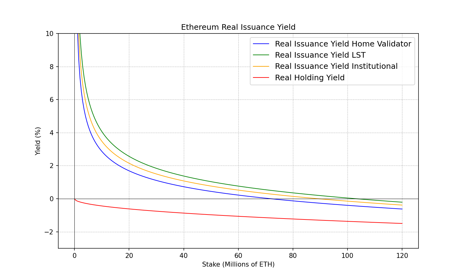
We can plot the real yield for the 4 different types of ETH stakeholders we introduced above, as a way to visualize the possible centralization forces that arise due to economies scale, and exogenous factors like taxes.
We can make the following observations, from which we will derive some consequences.
Observations
Observation 0: The economic choice to participate as a solo staker, LST holder, ETH holder or any other option is made on the gap between the real yields observed and the risks (liquidity, slashing, operational, regulatory, smart contract…) of each option. Typically higher risks demand a higher premium.
Observation 1: Holding always has a lower real yield than staking, at least for the assumptions taken above for costs. But the gap shrinks with high stake rates.
Observation 2: Different stakers cross the 0% real yield at different stake rate. Around 70M ETH staked solo validators start to earn negative real yield. At around 90M ETH institutional stakers start to earn negative real yield. At around 100M LST holders start to earn negative real yield.
Observation 3: When every staker and every ETH holder is becoming diluted (negative real yield), staking is a net cost for everyone.
Observation 4: There is quite a large gap between the stake levels where different stakers cross the 0% real yield.
Observation 5: Low nominal yields affect disproportionately home stakers over large operators. From the cost structure formula above we can see that as long as nominal yields are positive, the only term that can make the real yield negative is cc. This term is affected by economies of scale, and small operators will suffer larger cc.
Implications
Observation 0 and Observation 1 imply that as the gap between real yields becomes sufficiently small, participating in the network as some of those subsets may become economically irrational. For example, solo staking may be economically irrational given the operational risks, liquidity risks, slashing risks if the yield premium becomes sufficiently small vs holding. In that case solo stakers may become holders or switch to other forms of staking (e.g. LSTs) where the premium still satisfies the risk.
Together with Observation 2 and Observation 4 implies that as stake rates become higher and higher the chain is at risk of becoming more centralized, as solo stakers (which are the most uncorrelated staking set) must continue staking when it may be economically irrational to do so. Given the above assumptions LSTs will always observe at least 1% real yield higher than holding even at extreme stake rates (~100%), this may mean that there is always an incentive to hold an LST instead of ETH. Furthermore, when solo stakers cross to negative real yield but other stakers do not, other stakers are slowly but steadily gaining greater weight.
From Observation 3 we know that the very high stake rate regime, where everyone is observing a negative real yield, is costly for everyone. Everyone observes dilution. The money is going to the costs that were included in the real yield calculation (tax, ISPs, HW, electricity, labor…).
Observation 5 implies that nominal yield reductions need to be applied with care and certainly not in isolation without introducing uncorrelation incentives at the same time. As they risk penalizing home solo stakers disproportionately.
Recommendations
Given the above analysis, we can put forward a few recommended properties the yield curve (respectively the issuance curve) should have. The idea of establishing these properties is that we should be able to discuss them individually and agree or disagree on their desirability. Once agreed they constrain the set of functions we should consider. At a minimum, it will make the discussion about issuance changes more structured.
Property 0: Although this property is already satisfied with the current issuance curve, it is worth stating explicitly. The protocol should incentivize some minimum amount of stake, to ensure the network is secure and the cost to attack much larger than the potential economic reward of doing so. This is achieved by defining a yield curve that ramps up the nominal yield as the total proportion of stake (s_nsn) is reduced.
Property 1: The yield curve should contain uncorrelation incentives such that stakers are incentivized to spin-up uncorrelated nodes and to stake independently, instead of joining large-scale operators. From a protocol perspective the marginal value gained from another ETH staked through a large staking operation is much smaller than if that same ETH does so through an uncorrelated node. The protocol should reward uncorrelation as that’s what allows the network to achieve the extreme levels of censorship resistance, liveness/availability and credible neutrality the protocol expects to obtain from its validator set. The economic incentives must be aligned with the expected outcomes, therefore the yield curve must contain uncorrelation incentives.
Property 2: The issuance curve (resp. yield curve) should have a regime where holding is strictly more economically beneficial than staking, at sufficiently high stake rates. This means that the real yield of holding is greater than the real yield of staking if the stake rate is sufficiently high. As explained above it’s the real yield gap the defining characteristic that establishes the economically rational choice to join one subset or another. If the holding real yield can be greater than the staking real yield at sufficiently high stake rates there is an economic incentive to hold instead of continue staking. To be noted, up to here we are not making an argument at what stake rate this should be set. It suffices to agree that 99.9% stake rate is unhealthy for the protocol (it’s a cost for everyone, LSTs will displace ETH as pristine collateral, etc…). If that’s the case, then we can prevent this outcome by setting the holding real yield to be higher than staking at that level. Unhealthy levels are likely found at much lower values of stake rate.
Property 3: To prevent centralization forces, the stake rates at which uncorrelated validators vs correlated validators cross to negative real yield should be small, as small as possible. A large gap between the thresholds to negative real yields of uncorrelated (e.g. home stakers) and correlated sets (e.g. large operators) creates a regime where the validator set can become more and more centralized. To make the case more clear, if uncorrelated validators reach 0 real yield at 30M ETH staked, while holding an LST composed of large operators (e.g. cbETH, wstETH) does so at 100M ETH. The regime where the stake ranges between 30M and 100M is such that solo stakers will tend to disappear, either quickly (they stop staking) or slowly (they become more and more diluted), the outcome in either case is a more centralized validator set.
Property 4: The yield curve should taper down relatively quick to enter the regime of negative real yields. From Property 2 and Property 3 we know we should build-in a regime where the real yield from issuance goes negative, but we want this regime to occur approximately at the same stake rate for the different types of stakers, to prevent centralization forces. Observation 5 implies that if the slope of this nominal yield reduction is slow, stakers with different cost structures will be pushed out at much different stake rates. Hence, we need to make this yield reduction quick.
Property 5: The issuance yield curve should be continuous. It’s tempting to play with discontinuous yield curves, but yield is the main incentive to regulate the total stake of the network. We would like that the changes induced to the total stake ss are continuous, therefore the economic incentive should be a continuous function.
Exploring Other Issuance Curves
The desired properties can be summarized very succinctly:
- The yield curve should be continuous.
- The yield curve should go up as stake rate goes to 0.
- The yield curve should go to 0 as the stake rate goes up, crossing 0 at some point that bounds from above the desired stake rate equilibrium.
- The yield curve should have uncorrelation incentives such that spinning up uncorrelated validators is rewarded and incentivized over correlated validators.
- The real yield curves of correlated and uncorrelated stakers should become negative relatively close to each other.
A very simple solution to meet the above is to introduce a negative term to Ethereum’s issuance yield and uncorrelation incentives.
The negative term should grow faster than the issuance yield as the stake grows, so that it eventually overcompensates issuance and makes the yield go negative quickly at sufficiently high stake rates. This negative term can be thought of as a stake burn, and should be applied on a slot or epoch basis such that it’s unavoidable (thanks to A. Elowsson for this observation).
Uncorrelation incentives are being explored in other posts. We will simply leave here the recommendation of adopting them as part of any issuance tweaks. Read further: Anti-Correlation Penalties by Wahrstatter et al.
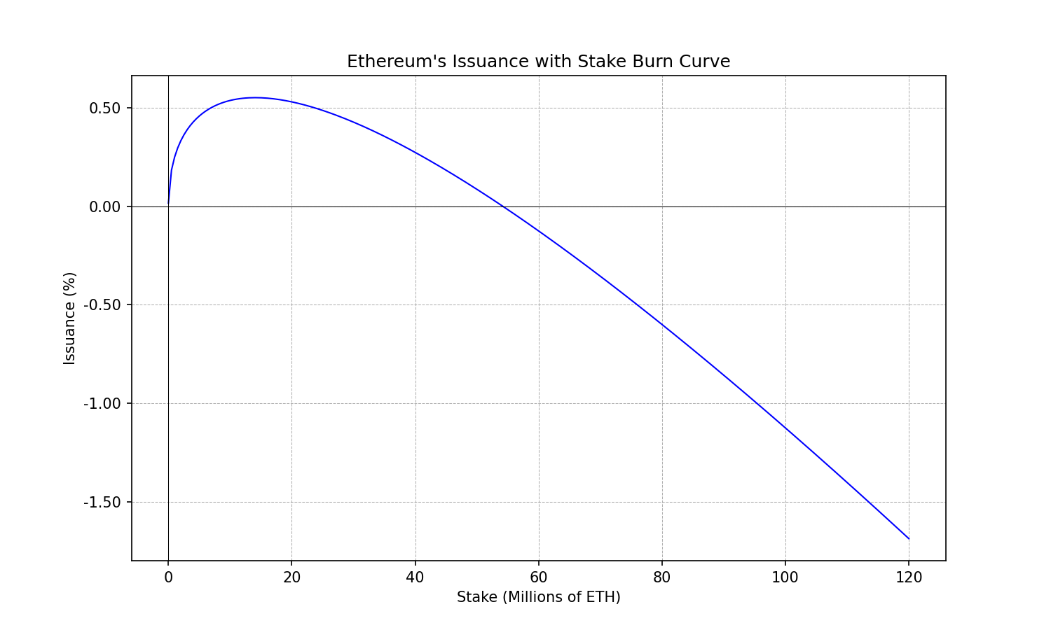
Ethereum’s Issuance with Stake Burn
The following is an example of how such a negative term can be introduced.
i(s) = 2.6 \cdot 64 \cdot \sqrt{s} - 2.6 \cdot \frac{s \ln s}{2048} \quad \text{ETH} \cdot \text{year}^{-1}i(s)=2.6⋅64⋅√s−2.6⋅slns2048ETH⋅year−1
y_{s}(s) = 1 + \frac{2.6 \cdot 64}{\sqrt{s}} - \frac{2.6 \ln s}{2048} \quad \text{year}^{-1}ys(s)=1+2.6⋅64√s−2.6lns2048year−1
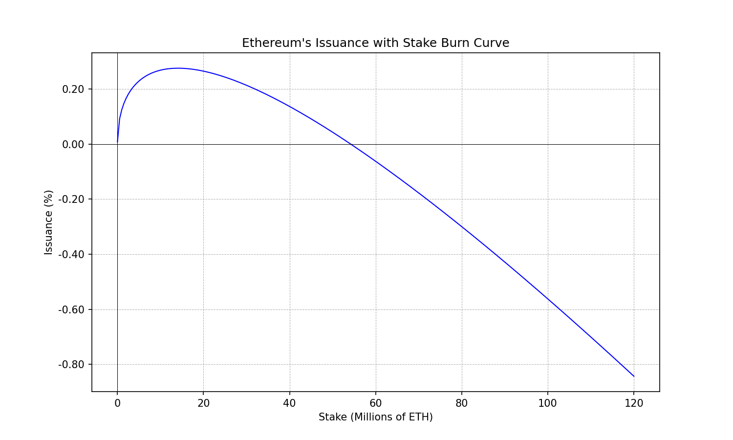
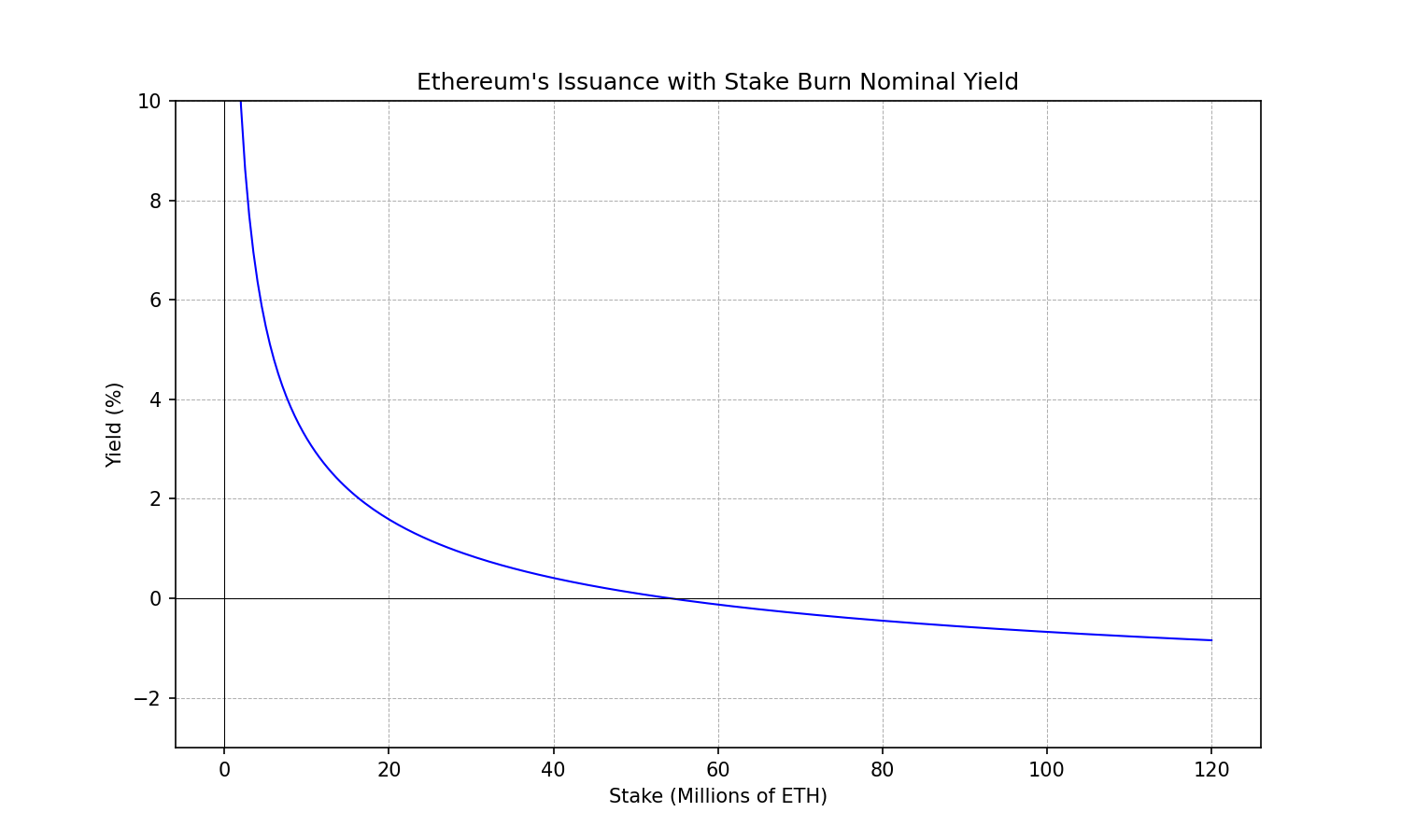
The negative stake burn term eventually dominates issuance and can make it go negative. There is complete freedom deciding where this threshold occurs, by simply tweaking the constant pre-factors. In this particular case, the parameters have been chosen so they are rounded in powers of 2 and so that the negative issuance regime roughly happens around 50% stake rate.
This negative issuance regime induces a positive effective yield on holders, which provides the protocol with an economic incentive to limit the stake rate. As the real yield will eventually be greater holding ETH than staking. It also serves to protect the network from overloading its consensus layer, as it provides the protocol with a mechanism to charge exogenous sources of yield that occur on top of it. If priority fees, MEV, or restaking provide additional yield that would push stake rates above the desired limit, the protocol would start charging those extra sources of yield by making issuance go negative. Hence redistributing exogenous yield onto ETH holders.
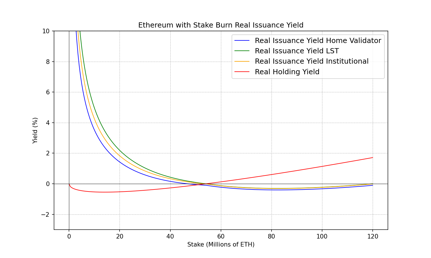
To understand better the impact that this stake burn has on the different stakeholders we can plot the real yield curves.
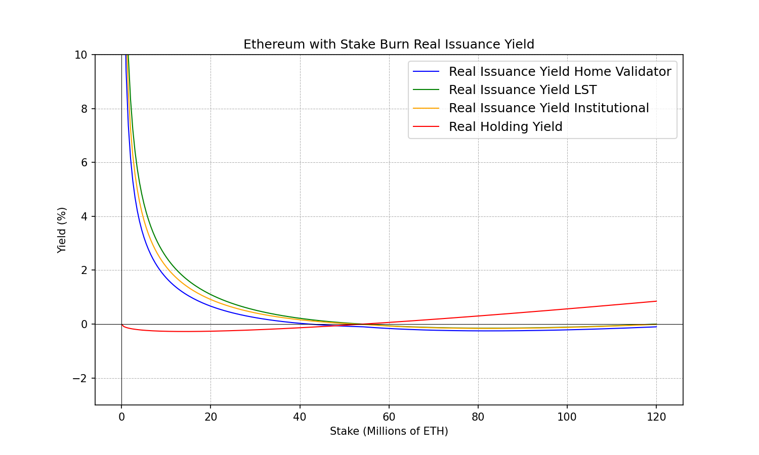
We can see how the introduction of a negative issuance yield regime has helped achieve most of the properties we desired to obtain. Particularly, we can notice the stake rates at which different stakeholders reach 0 real yield have compressed and are much closer to each other. And we can appreciate how when stake rates get close to 50% (given the choice of parameters) holders start to observe a positive real yield which disincentivizes additional staking. Holding real yields can become quite large so even large exogenous sources of yield can be overcome.
Given that we haven’t touched the positive issuance term, this results in a large reduction of the staking yield. We can increase the yield trivially while respecting the same yield curve shape. Here the same curve with larger yield:
i(s) = 2.6 \cdot 128 \cdot \sqrt{s} - 2.6 \cdot \frac{s \ln s}{1024} \quad \text{ETH} \cdot \text{year}^{-1}i(s)=2.6⋅128⋅√s−2.6⋅slns1024ETH⋅year−1
y_{s}(s) = 1 + \frac{2.6 \cdot 128}{\sqrt{s}} - \frac{2.6 \ln s}{1024} \quad \text{year}^{-1}ys(s)=1+2.6⋅128√s−2.6lns1024year−1
This shows the target yield that is observed at a specific stake rate is a separate consideration to the curve shape discussion. So if you dislike this particular example because of the resulting yield at current stake rates. Fear not, that has an easy fix.
Adding Uncorrelation Incentives to the Mix
We will not cover the specifics of how uncorrelation incentives should be introduced nor how they should be sized, but we will illustrate how the introduction of a correlation penalty can help align the economic incentives with the network interest of maintaining an uncorrelated validator set.
To do so we will simulate what would happen to the real yields observed by the following stakeholders:
- Home Validator (Very Uncorrelated): -0.0% subtracted to the nominal yield through correlation penalties
- LST Holder through a decentralized protocol (Quite Uncorrelated): -0.2% subtracted to the nominal yield through correlation penalties
- LST Holder through staking through large operators (Quite Correlated): -0.4% subtracted to the nominal yield through correlation penalties
- Large Institutional Operator (Very Correlated): -0.6% subtracted to the nominal yield through correlation penalties
The following figure zooms in to the area where negative real yields are achieved:
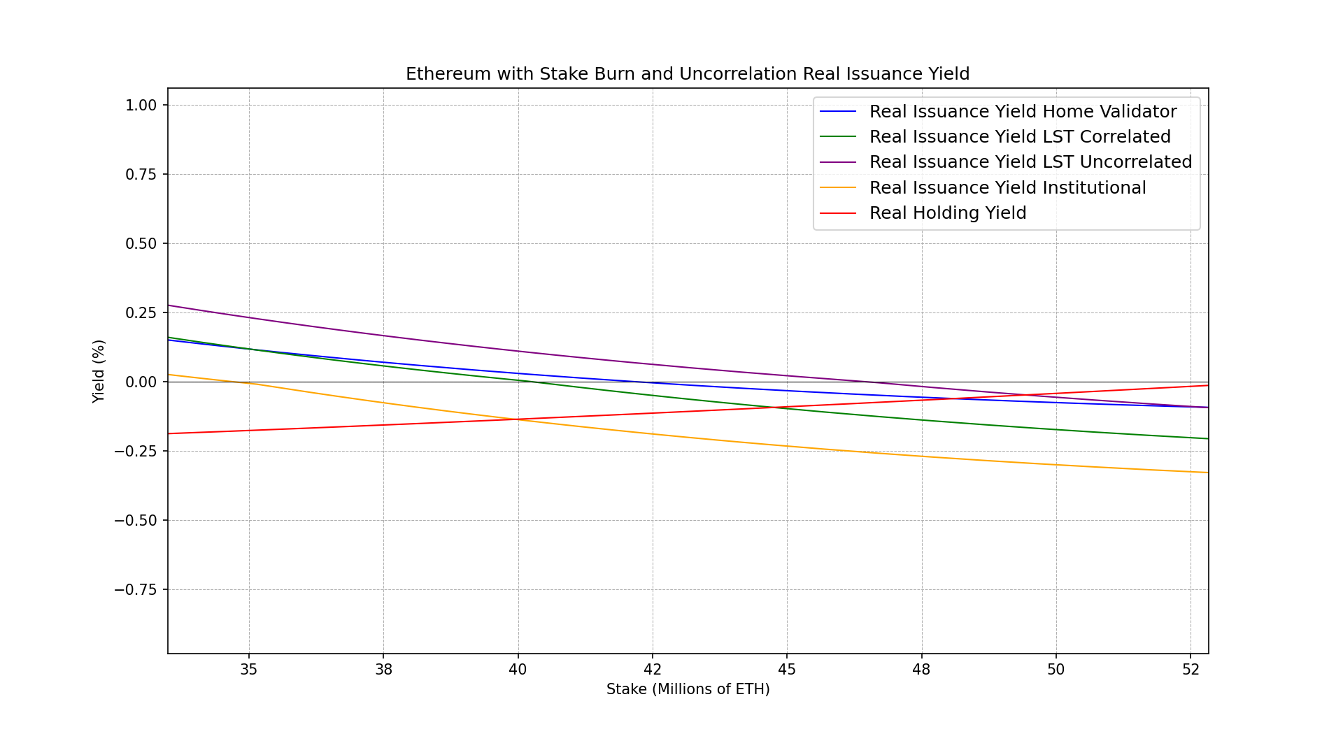
Important Note: The above values for correlation penalties are not based on any estimation or study. They have been chosen arbitrarily to showcase that the inclusion of uncorrelation incentives in the issuance curve can be used to disincentivize staking through large correlated operators. We refer the analysis of the right incentives to other papers.
Fixing the Issuance Yield Curve
Up until now the focus has been on the shape of the yield curve (respectively the issuance curve) but very little has been said about the specific yield we should target at different stake rates. As illustrated above, by simply applying a multiplicative factor we can keep the same curve shape but make yields be higher or lower as wished.
In this section we will provide some heuristic properties to address this problem and be able to specify the prefactors that allow us to define a concrete yield curve.
These heuristic properties are orientative. There is no hard science behind them, just some soft arguments that provide reasonable justification for these choices.
Heuristic 0: The nominal issuance yield should become negative at 50% stake rate or lower. Higher stake rates start to become problematic, above those levels the majority of circulating supply is staking. In case of supermajority bug the majority of ETH holders could be incentivized to break the consensus rules. The negative yield regime can be seen as a protection mechanism from the protocol to prevent this type of situations from happening, it sets an economic incentive to align the social layer with the protocol interests.
Heuristic 1: Target 3% yield at 25% stake rate. When PoS was released there was no idea what would be the expected staking yield the market would consider appetizing. Would 5% be enough? Or 3%?
Now we have data points, current staking yield is 3% as measured by https://beaconcha.in (issuance, MEV, and priority fees included). So we know the market certainly has appetite for ETH yield at 3%. There is also some soft-arguments by V. Buterin, J. Drake et al. that 25% stake rate should provide enough security.
And finally, the current issuance curve happens to provide 3% yield at 25% stake rate. So by fixing the new curve to meet that same yield at 25% we anchor the same yield (and issuance) at the target rate. But any extra amount of stake will be met with a reduction in yield and issuance that makes it go to 0 before hitting 50%.
As current stake rate is a tad over 25% the proposed change to the issuance curve would imply a bit of issuance reduction, nothing very significant. But most importantly it avoids the ever growing issuance increase as stake rates become higher.
In conjunction with well designed uncorrelation incentives it could help the protocol ensure it does not overpay for security, stake rates are self-limiting, and the validator set very uncorrelated.
Final Words
The analytic form of the yield curve or the issuance curve matter much less than we may think. It might be tempting to spend time tinkering with its concrete analytic form but for all it matters it could be equally defined with a piece-wise continuous function.
Its purpose is to provide an economic incentive to get stake rates where the protocol needs them to be (not too high, not too low) and maintaining a large uncorrelated validator set.
This post is an invitation to steer the discussion towards said properties instead of getting lost with the fine details. If we nail down the properties we will constrain the solution space enough so that almost any function we choose will do the job.