Author: @BlazingKevin_ , the Researcher at Movemaker

In the cryptoasset market, traders often encounter two typical issues: a significant discrepancy between the bid and ask prices of the target token; and drastic price fluctuations after submitting large market orders, resulting in significant deviations from expected prices and high slippage costs. Both of these issues stem from a common underlying factor: insufficient market liquidity. Market makers are key players in systematically addressing this issue.

The precise definition of a market maker is a professional quantitative trading company whose core business is to continuously and simultaneously submit intensive buy (Bid) and sell (Ask) quotes around the current market price of an asset on the exchange's order book.

Their fundamental function is to provide continuous liquidity to the market. By providing two-sided quotes, market makers directly narrow the bid-ask spread and increase the depth of the order book. This ensures that other traders' buy and sell orders are instantly matched at any given time, enabling efficient and fair trade execution. Market makers profit from the small spreads they capture across a large trading volume, as well as from fees paid by exchanges to incentivize liquidity provision.

The market conditions of October 11th have brought the role of market makers to the forefront of market discussion. When prices fluctuate dramatically, a key question arises: Do market makers passively trigger cascading liquidations, or do they proactively withdraw liquidity offers when risks intensify?

To analyze market makers’ behavior in similar situations, it’s necessary to first understand the fundamental principles of their operations. This article aims to systematically answer the following core questions:

1. What is the business model that market makers rely on to make profits?
2. What quantitative strategies do market makers adopt to achieve their business goals?
3. When market volatility intensifies and potential risks emerge, which risk control mechanisms will market makers activate?

Based on clarifying the above issues, we will be able to more clearly infer the behavioral logic and decision-making trajectory of market makers in the 1011 market.

Market Maker's Basic Profit Model

1.1 Core Profit Mechanism: Price Difference Capture and Liquidity Rebate

To understand the behavior of market makers in the market, we must first understand their fundamental source of profit. Market makers provide continuous two-sided quotes on the exchange's order book (i.e., "market making"). Their profits primarily come from two sources: capturing the bid-ask spread and earning commissions from the exchange's liquidity provision .

To illustrate this mechanism, we construct a simplified contract order book analysis model.

Source: Movemaker

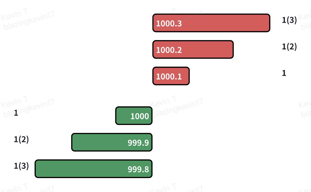
Assume there is an order book with the following order distribution:

• Bids : Densely distributed at price levels such as $1000.0, $999.9, and $999.8.
• Asks : Densely distributed at price levels such as $1000.1, $1000.2, and $1000.3.

At the same time, we set the following market parameters:

• Single-party handling fee : 0.02%
• Order maker commission : 0.01%
• Minimum price increment : $0.1
• Current Spread : The difference between the best bid price ($1000.0) and the best ask price ($1000.1) is $0.1.

1.2 Transaction Process and Cost-Benefit Analysis

Now, let’s break down the market maker’s revenue process through a complete trading cycle.

Step 1: Market Maker’s Buy Order is Passively Executed (Taker Sells)

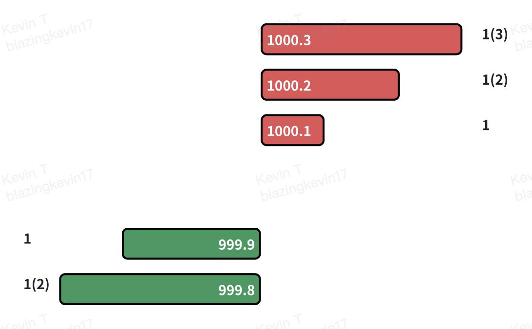
Source: Movemaker

• Event : A trader (Taker) sells a contract at the market price. This order is matched by the best limit buy order in the order book, which is a buy order placed by the market maker at $1000.0 .
• Notional Cost : From the transaction record, it seems that the market maker established a long position of one contract at a price of $1000.0.
• Effective Cost : However, since the market maker is acting as a liquidity provider (Maker), not only does this trade not incur any fees, but it also receives a 0.01% commission from the exchange. In this example, the commission is $1000.00 * 0.01% = $0.10. Therefore, the market maker's actual outflow (effective cost) for establishing this long position is: $1000.00 (notional cost) - $0.10 (rebate) = $999.90 .

Step 2: Market Maker’s Sell Order is Passively Executed (Taker Buys)

• Event : A trader (Taker) buys one contract at the market price. This order is matched by the best limit sell order in the order book, a sell order placed by the market maker at $1000.1 . This closes the long position established by the market maker in step 1.
• Notional Income : The transaction record shows that the market maker sold at a price of $1000.1.
• Effective Income : Similarly, as the liquidity provider, the market maker receives another 0.01% commission on this sell transaction, resulting in $1000.1 * 0.01% ≈ $0.1. Therefore, the market maker's actual inflow (effective income) from closing the position is: $1000.1 (notional income) + $0.1 (rebate) = $1000.2 .

1.3 Conclusion: Composition of Real Profit

By completing this complete cycle of buying and selling, the market maker’s total profit per transaction is:

Total revenue = effective revenue − effective cost = $1000.2 − $999.9 = $0.3

This shows that the market maker’s real profit is not just the $0.1 nominal spread visible on the order book. Its real profit is composed of:

Real profit = nominal price difference + buy order rebate + sell order rebate

$0.3=$0.1+$0.1+$0.1

This model of accumulating tiny profits by repeating the above process countless times in high-frequency trading constitutes the most basic and core profit model of market maker business.

Market Makers’ Dynamic Strategies and Risk Exposure

2.1 Challenges of Profit Models: Directional Price Changes

The aforementioned basic profit model is premised on the assumption that market prices fluctuate within a narrow range. However, when the market experiences a clear, unilateral, directional movement, the model faces severe challenges and exposes market makers to a core risk: adverse selection .

Adverse selection means that when new information enters the market and causes the fair value of an asset to change, informed traders will selectively execute quotes that have not been updated by the market maker and are at the "wrong" price, thereby causing the market maker to accumulate a position that is unfavorable to it.

2.2 Scenario Analysis: Strategic Choices for Dealing with Price Declines

To illustrate, we continue with the previous analysis model and introduce a market event: the fair price of an asset drops rapidly from $1000 to $998.0.

Source: Movemaker

Assume the market maker holds only one long contract, established in a previous transaction, with an effective cost of $999.9. If the market maker takes no action, its open buy orders near $1000.0 will present a risk-free profit opportunity for arbitrageurs. Therefore, upon detecting a directional price movement, the market maker must react immediately, initially canceling all buy orders close to the old market price .

At this point, the market maker faces a strategic choice, with three main options:

• Option 1: Close the position immediately and realize the loss. The market maker can choose to sell the long contract immediately with a market order. Assuming the transaction is completed at $998.0, the market maker will be charged a taker fee of 0.02%.

  Loss = (Effective Cost − Exit Price) + Taker Fee

  Loss = ($999.9 − $998.0) + ($998.0 × 0.02%) ≈ $1.9 + $0.2 = $2.1

  The purpose of this option is to quickly eliminate risk exposure, but it will immediately result in a certain loss.

• Option 2: Adjust the Quote to Seek a Better Exit Price. The market maker can lower its sell price to near the new fair market price, for example, $998.1. If the sell order is executed, the market maker will receive a commission as the order maker.

  Loss = (Effective Cost − Exit Price) − Order Rebate

  Loss = ($999.9 − $998.1) − ($998.1 × 0.01%) ≈ $1.8 − $0.1 = $1.7

  This strategy aims to exit a position with a smaller loss.

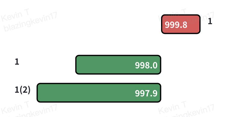
• Option 3: Widen the Spread to Manage Existing Positions . Market makers can adopt an asymmetric quote strategy: adjusting the ask price to a relatively unattractive level (as shown in the figure, $998.8) while simultaneously placing new buy orders at lower levels (such as $998.0 and $997.9). This strategy aims to manage and reduce the average cost of existing positions through subsequent trades.

2.3 Strategy Execution and Inventory Risk Management

Assuming a "single market maker" market structure, given its absolute pricing power, the market maker would likely choose option three to avoid immediate losses. In this option, since the sell order price ($998.8) is significantly higher than the fair price ($998.0), its probability of being filled is low. Conversely, a buy order ($998.0), which is closer to the fair price, is more likely to be filled by a seller in the market.

Step 1: Reduce average cost by increasing holdings

• Event : The buy order placed by the market maker at $998.0 is filled.
• Effective cost of new position : $998.0 - (998.0×0.01%)≈$997.9
• Updated total position : The market maker now holds two long contracts, with a total effective cost of $999.9 + $997.9 = $1997.8.
• Updated average cost : $1997.8 / 2 = $998.9

Step 2: Adjust your quote based on the new costs

Through these actions, the market maker successfully lowered the breakeven point for its long position from $999.9 to $998.9. With this lower cost base, the market maker can now more actively pursue selling opportunities. For example, it can significantly lower the ask price from $998.8 to $998.9 , achieving breakeven while significantly narrowing the spread from $1.8 ($999.8 - $998.0) to $0.8 ($998.8 - $998.0) to attract buy orders.

2.4 Limitations of the Strategy and Risk Exposure

However, this strategy of diluting costs by increasing holdings has clear limitations. If prices continue to fall, for example, from $1,000 to $900, market makers will be forced to continue increasing their holdings despite continued losses, dramatically increasing their inventory risk . At that point, the widening spread will lead to a complete trading halt, forming a vicious cycle that ultimately forces them to close their positions at a significant loss.

This leads to a deeper question: How do market makers define and quantify risk? And what core factors are associated with different levels of risk? Answering these questions is key to understanding their behavior in extreme markets.

Core risk factors and dynamic strategy formulation

Market makers' profit model essentially involves assuming specific risks in exchange for returns. Losses they face primarily stem from significant short-term deviations in asset prices that are unfavorable to their inventory positions. Therefore, understanding their risk management framework is key to analyzing the logic behind their behavior.

3.1 Identification and Quantification of Core Risks

The risks faced by market makers can be summarized into two core interrelated factors:

1. Market volatility : This is the primary risk factor. Increased volatility means that the likelihood and magnitude of price deviations from the current mean increase, directly threatening the value of market makers' inventory.
2. Speed of mean reversion : This is the second key factor. The speed with which prices return to equilibrium after a deviation determines whether market makers will eventually profit by flattening their costs or suffer persistent losses.

A key observable indicator for determining the likelihood of mean reversion is trading volume . In my article, "A Review of Intensified Market Divergence: Is the Rally Transforming into a Reversal, or a Second Distribution of the Downtrend?" published on April 22nd of this year, I discussed the marble theory within the order book. Orders at different prices form layers of glass of varying thickness based on their volume, likening a volatile market to a marble. Limit orders at different prices on the order book can be viewed as having "liquidity absorption layers" of varying thickness.

Short-term market price fluctuations can be thought of as a force acting as a marble. In low-volume environments, this force is weak, and prices are typically confined to a narrow range within the densest layers of liquidity. In high-volume environments, however, this force is intensified, powerful enough to penetrate multiple layers of liquidity. Depleted liquidity layers are difficult to replenish instantly, especially in one-sided markets. This leads to persistent price movement in one direction, reducing the probability of mean reversion. Therefore, trading volume per unit time is an effective proxy for the strength of this force .

3.2 Dynamic Strategy Parameterization Based on Market Status

Source: Movemaker

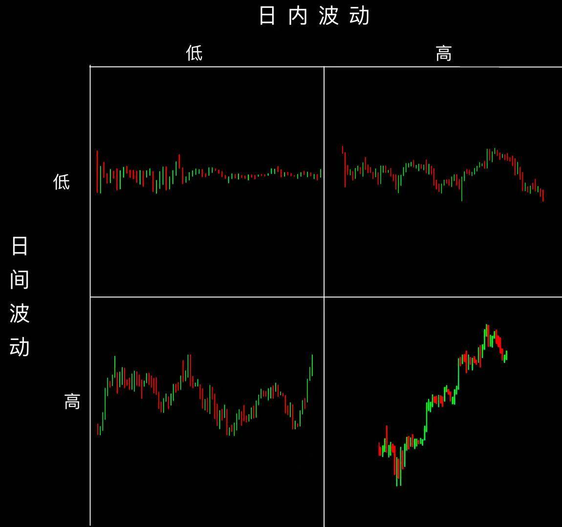
Based on the performance of volatility on different time scales (intraday vs. intraday), market makers will dynamically adjust their strategy parameters to adapt to different market environments. Their basic strategies can be summarized into the following typical states:

• In stable markets , when intraday and day-to-day price volatility is low, market makers tend to be very aggressive, using large orders and tight spreads , aiming to maximize trading frequency and market share to capture as much volume as possible in a low-risk environment.

• In a range-bound market , when prices exhibit high intraday volatility but low interday volatility, market makers are more confident that prices will revert to the short-term mean. Consequently, they widen spreads to maximize profits while maintaining larger order sizes to ensure sufficient liquidity to mitigate losses during price fluctuations.

• In trending markets , when prices fluctuate smoothly intraday but exhibit a clear, one-way trend during the day, market makers' risk exposure increases dramatically. At this point, their strategies shift to defensive strategies. They employ extremely narrow spreads and small order sizes , aiming to quickly execute orders to capture liquidity and quickly exit with stop-loss orders if the trend turns against their inventory, thus avoiding fighting the long-term trend.

• In extremely volatile markets (crisis states) , when intraday and interday price volatility increases across the board, market makers' risk management becomes paramount. Strategies become extremely conservative, with significantly widened spreads and small order sizes employed to manage inventory risk with extreme caution. In this high-risk environment, many competitors may withdraw, leaving potential opportunities for market makers with the ability to manage risk effectively.

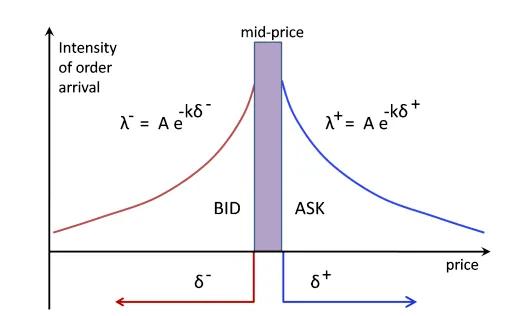
3.3 The Core of Strategy Execution: Fair Price Discovery and Spread Setting

Regardless of market conditions, the execution of market maker strategies revolves around two core tasks: determining fair prices and setting optimal spreads .

1. Determining a fair price is a complex question with no single correct answer. If the model is incorrect, the market maker's quotes can be "eaten up" by better-informed traders, causing them to systematically accumulate losing positions. Common basic approaches include using an index price aggregated across multiple exchanges or taking the midpoint of the current best bid and ask prices. Ultimately, regardless of the model employed, market makers must ensure that their quotes are competitive and can effectively liquidate inventory. Holding large, one-sided positions for extended periods of time is the primary cause of significant losses.

2. Setting the optimal spread is even more challenging than discovering the fair price, as it involves a dynamic, multi-party process. Overly aggressively narrowing the spread can lead to a "competitive equilibrium trap": while securing the best quote position, profit margins are squeezed, and arbitrageurs are easily preempted in price fluctuations. This requires market makers to develop a more intelligent quantitative framework.

3.4 A Simplified Optimal Spread Quantification Framework

To illustrate its internal logic, we quote a simplified model constructed by David Holt , the author of Meduim, to derive the optimal spread under a highly idealized assumption.

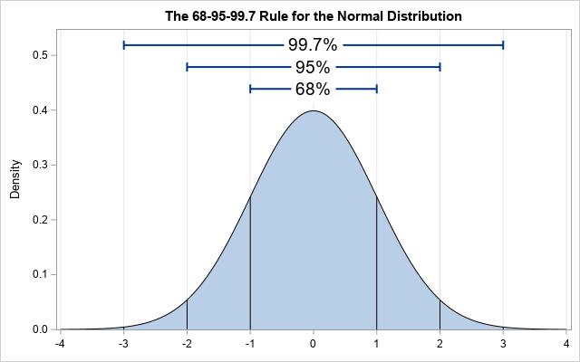
• A. Core Assumptions and Volatility Calculation: Assuming that market prices follow a normal distribution in the short term, we examine a 60-second sample of data with a 1-second sampling period. We calculate the standard deviation (σ) of the mark price within this sample relative to the average mid-price to be $0.4 . This means that approximately 68% of the time, the next-second price will fall within the range [mean - $0.4, mean + $0.4].

Source: Idrees

• B. Correlating Spreads, Probabilities, and Expected Returns Based on this, we can infer the probability of execution at different spreads and calculate their expected returns. For example, if we set a spread of $0.8 (i.e., placing orders at $0.4 on either side of the mean), the price must fluctuate at least one standard deviation to trigger the order, with a probability of approximately 32%. Assuming each trade captures half the spread ($0.4), the expected return per time period is approximately $0.128 (32% × $0.4).

Source: Zhihu

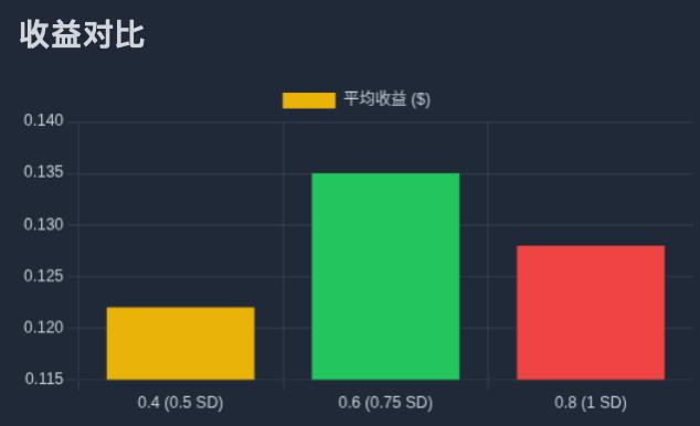
• C. Finding the Optimal Solution By iteratively calculating different spreads, we found that a spread of $0.2 yields an expected return of approximately $0.08; a spread of $0.4 yields an expected return of approximately $0.122; a spread of $0.6 yields an expected return of approximately $0.135; and a spread of $0.8 yields an expected return of approximately $0.128. The conclusion is that under this model, the optimal spread is $0.6 , meaning placing an order at a distance of $0.3 (approximately 0.75σ) from the average price maximizes expected returns.

Source: Movemaker

3.5 From Static Models to Dynamic Reality: Multi-Time Frame Risk Management

The fatal flaw of the above model is its assumption of a constant mean . In real markets, price averages drift over time. Therefore, professional market makers must employ a multi-timeframe , layered strategy to manage risk.

The core of this strategy lies in using quantitative models to set optimal spreads at the micro level (seconds), while simultaneously monitoring price mean drift and changes in volatility structure at the meso level (minutes) and macro level (hours/days). When the mean shifts, the system dynamically recalibrates the central axis of the entire quote range and adjusts inventory positions accordingly.

This layered model ultimately leads to a set of dynamic risk control rules:

1. Automatically widen the spread when second-by-second volatility increases .
2. When medium-term volatility increases, reduce the size of individual orders but increase the number of order levels to spread inventory over a wider price range.
3. When the long-term trend is opposite to the direction of inventory positions, active intervention is carried out , such as further reducing the size of pending orders or even suspending the strategy to prevent systemic risks.

Risk response mechanisms and advanced strategies

4.1 Inventory Risk Management in High-Frequency Market Making

The dynamic strategy model described above falls under the category of high-frequency market making . The core goal of this type of strategy is to use algorithms to set optimal buy and sell quotes to maximize expected profits while accurately managing inventory risk .

Inventory risk is defined as the exposure of a market maker to adverse price fluctuations due to holding a net long or net short position. When a market maker holds a long position in inventory, they risk losses from falling prices; conversely, when they hold a short position in inventory, they risk losses from rising prices. Effectively managing this risk is crucial to a market maker's long-term survival.

Professional quantitative models, such as the classic Stoikov model , provide a mathematical framework for understanding risk management. This model aims to proactively manage inventory risk by calculating a dynamically adjusted "reference price." Market makers' bilateral quotes revolve around this new reference price, rather than the static market midpoint. The core formula is as follows:

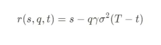
The meaning of each parameter is as follows:

• r(s,q,t): The dynamically adjusted reference price, which is the benchmark axis for market makers' quotes.
• s: current market median price.
• q: Current inventory. Positive if long, negative if short.
• γ: Risk aversion parameter. This is a key variable set by market makers to reflect their current risk appetite.
• σ: volatility of the asset.
• (T−t): The remaining time until the end of the trading cycle.

The core idea of this model is that when a market maker's inventory (q) deviates from its target (usually zero), the model systematically adjusts the quote axis to incentivize market execution of orders that will bring its inventory back to equilibrium. For example, when holding a long position (q>0), the model's calculated r(s,q,t) will be lower than the market midpoint s. This means that the market maker will shift its bid and ask quotes downward, making sell orders more attractive and buy orders less attractive, thereby increasing the probability of closing out the long position.

4.2 Risk Aversion Parameter (γ) and the Final Choice of Strategy

The risk aversion parameter γ is the "regulating valve" of the entire risk management system. Market makers dynamically adjust the value of γ based on a comprehensive assessment of market conditions (such as volatility expectations and macroeconomic events). During stable market conditions, γ may be low, favoring an aggressive strategy to profit from price differences. When market risk intensifies, γ is adjusted higher, making the strategy extremely conservative, with quotes deviating significantly from the mid-price to rapidly reduce risk exposure.

In extreme cases, when the market signals the highest level of risk (e.g., liquidity drying up, a sharp price decoupling), γ can become extremely large. In these cases, the model's optimal strategy may generate a quote that deviates significantly from the market and is virtually impossible to execute. In practice, this is equivalent to a rational decision— temporarily and completely withdrawing liquidity to avoid catastrophic losses due to uncontrollable inventory risk.

4.3 Complex Strategies in Real Life

Finally, it must be emphasized that the model discussed in this article merely illustrates the core logic of market makers under simplified assumptions. In a real, highly competitive market environment, top market makers employ a far more complex, multi-layered combination of strategies to maximize profits and manage risk.

These advanced strategies include, but are not limited to:

• Hedging strategies : Market makers typically do not leave their physical inventory exposed to risk. Instead, they will establish opposite positions in derivatives markets such as perpetual contracts, futures, or options to achieve delta-neutral or more complex risk exposure management, shifting their risk from price direction risk to other controllable risk factors.

• Specialized Execution : In certain scenarios, the role of market makers goes beyond passive liquidity provision. For example, after a project's TGE, they sell a large number of tokens within a certain period of time through strategies such as TWAP (Time Weighted Average Price) or VWAP (Volume Weighted Average Price) , which constitutes a significant source of profit for them.

1011 Review: Risk Triggering and the Inevitable Choice of Market Makers

Based on the analytical framework established above, we can now revisit the market volatility of October 11th. When prices exhibit a dramatic one-way movement, the market maker's internal risk management system is inevitably triggered. This system may be triggered by a combination of factors: average losses within a specific timeframe exceeding a preset threshold; net inventory positions being "filled" by market counterparties in a very short period of time; or, after reaching the maximum inventory limit, the inability to effectively liquidate positions, leading to the system's automatic position reduction process.

5.1 Data Analysis: Structural Collapse of the Order Book

To understand the true state of the market at the time, we must delve into the microstructure of the order book. The following chart, taken from an order book visualization tool, provides us with evidence:

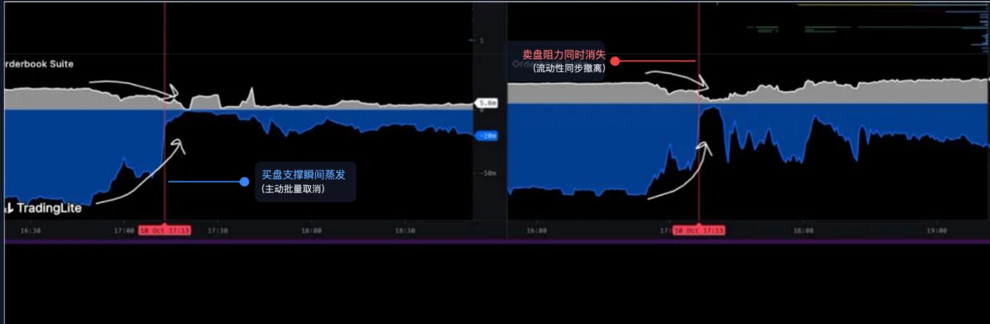
Source: @LisaLewis469193

(Note: To maintain the rigor of the analysis, please regard this chart as a typical representation of the market conditions at the time)

This chart visually shows how order book depth has changed over time:

• Gray area : represents sell liquidity, which is the total amount of limit orders waiting to be sold above the current price.
• Blue/black area : represents buy liquidity, that is, the total amount of limit orders waiting to be bought below the current price.

At the precise moment of 5:13 AM, marked by the red vertical line in the image, we can observe two unusual and simultaneous phenomena:

1. The instantaneous evaporation of buying support : A massive, nearly vertical "cliff" appears in the blue area below the chart. This pattern is completely different from a situation where buy orders are consumed by a large number of trades—the latter would show a gradual, step-by-step erosion of liquidity. The only plausible explanation for this uniform vertical disappearance is the active, simultaneous, and wholesale cancellation of a large number of limit buy orders .
2. The simultaneous disappearance of selling resistance : an almost identical “cliff” appeared in the gray area above the chart. A large number of limit sell orders were actively withdrawn at the same moment.

This series of actions, known in trading jargon as a " liquidity withdrawal ," signifies that the market's major liquidity providers (primarily market makers) have almost synchronously withdrawn their bilateral quotes within a very short period of time, instantly transforming a seemingly liquid market into an extremely fragile " liquidity vacuum ."

5.2 Two Phases of the Event: From Active Evacuation to Vacuum Formation

Therefore, the 1011 plunge can be clearly divided into two logically progressive stages:

Phase 1: Proactive, Systematic Execution of Risk Aversion

Before 5:13 a.m., the market may still be in a state of superficial stability. But at that moment, a key risk signal was triggered - this could be a breaking macro news or the on-chain risk model of a core protocol (such as USDe/LSTs) sounded an alarm.

Upon receiving the signal, the algorithmic trading system of the top market maker immediately executed a pre-set " emergency hedging procedure ." This procedure has a single goal: to minimize its own market risk exposure in the shortest possible time, taking precedence over any profit targets.

• Why cancel buy orders? This is a crucial defensive move. Market makers' systems predict that an unprecedented sell-off is imminent. If they don't immediately cancel their buy orders, they will become the market's "first line of defense," forcing them to take on a large amount of assets that are about to plummet, resulting in catastrophic inventory losses .

• Why cancel sell orders at the same time? This is also based on strict risk control principles. In an environment where volatility is about to surge, retaining sell orders carries risks (for example, the price could experience a brief upward "false breakout" before a sharp drop, causing sell orders to be executed prematurely at unfavorable prices). Within an institutional-level risk management framework, the safest and most rational option is to " clear all quotes and enter observation mode " until market predictability returns, then re-deploy strategies based on new market conditions.

Phase 2: The formation of a liquidity vacuum and the free fall of prices

After 5:13 a.m., as the order book "cliff" formed, the market structure underwent a fundamental qualitative change and entered a state of " liquidity vacuum " as we described.

Before an active retreat, a 1% drop in market price might require a large number of sell orders to consume the accumulated buying. However, after a retreat, since the underlying support structure no longer exists, only a very small number of sell orders may be needed to cause an equal or even greater price shock.

in conclusion

The epic market crash of October 11th was directly triggered and amplified by a massive, synchronized, proactive liquidity withdrawal by top market makers, as the chart reveals. They weren't the "culprits" or initiators of the crash, but they were its most effective " executors " and " amplifiers ." Through rational, self-preservation-focused collective actions, they created an extremely fragile "liquidity vacuum," perfecting the conditions for subsequent panic selling, pressure from protocol decoupling, and ultimately, a cascading liquidation of centralized exchanges.

About Movemaker

Movemaker, the first official community organization authorized by the Aptos Foundation and co-founded by Ankaa and BlockBooster, is dedicated to promoting the development of the Aptos ecosystem in the Chinese-speaking region. As the official representative of Aptos in the Chinese-speaking region, Movemaker is committed to building a diverse, open, and prosperous Aptos ecosystem by connecting developers, users, capital, and numerous ecosystem partners.

Disclaimer:

This article/blog is for informational purposes only and reflects the author's personal views and does not necessarily represent the views of Movemaker. This article is not intended to provide: (i) investment advice or a recommendation; (ii) an offer or solicitation to buy, sell, or hold digital assets; or (iii) financial, accounting, legal, or tax advice. Holding digital assets, including stablecoins and NFTs, carries significant risk and can experience significant price volatility and potentially become worthless. You should carefully consider whether trading or holding digital assets is appropriate for you based on your financial circumstances. If you have questions regarding your specific situation, please consult your legal, tax, or investment advisor. The information provided in this article (including market data and statistics, if any) is for general informational purposes only. While reasonable care has been taken in compiling these data and charts, no liability is assumed for any factual errors or omissions contained therein.